Tài liệu Hard Disk Drive Servo Systems- P2 docx

34 2 System Modeling and Identification
Structured model
with unknowns,
Input signal,
Actual plant
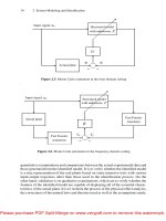
Figure 2.5. Monte Carlo estimation in the time-domain setting
.
Structured model
Input signal,
transform
with unknowns,
Actual plant
Fast Fourier
Fast Fourier
transform
Figure 2.6. Monte Carlo estimation in the frequency-domain setting
.
quantitative examinations and comparisons between the actual experimental data and
those generated from the identified model. It is to verify whether the identified model
is a true representation of the real plants based on some intensive tests with various
input-output responses other than those used in the identification process. On the
other hand, validation is on qualitative examinations, which are to verify whether the
features of the identified model are capable of displaying all of the essential charac-
teristics of the actual plant. It is to recheck the process of the physical effect analysis,
the correctness of the natural laws and theories used as well as the assumptions made.
Please purchase PDF Split-Merge on www.verypdf.com to remove this watermark.
2.4 Physical Effect Approach with Monte Carlo Estimations 35
In conclusion, verification and validation are two necessary steps that one needs
to perform to ensure that the identified model is accurate and reliable. As mentioned
earlier, the above technique will be utilized to identify the model of a commercial
microdrive in Chapter 9.

Please purchase PDF Split-Merge on www.verypdf.com to remove this watermark.
3
Linear Systems and Control
3.1 Introduction
It is our belief that a good unambiguous understanding of linear system structures,
i.e. the finite and infinite zero structures as well as the invertibility structures of lin-
ear systems, is essential for a meaningful control system design. As a matter of fact,
the performance and limitation of an overall control system are primarily dependent
on the structural properties of the given open-loop system. In our opinion, a control
system engineer should thoroughly study the properties of a given plant before carry-
ing out any meaningful design. Many of the difficulties one might face in the design
stage may be avoided if the designer has fully understood the system properties or
limitations. For example, it is well understood in the literature that a nonminimum
phase zero would generally yield a poor overall performance no matter what design
methodology is used. A good control engineer should try to avoid these kinds of
problem at the initial stage by adding or adjusting sensors or actuators in the system.
Sometimes, a simple rearrangement of existing sensors and/or actuators could totally
change the system properties. We refer interested readers to the work by Liu et al.
[70] and a recent monograph by Chen et al. [71] for details.
As such, we first recall in this chapter a structural decomposition technique of
linear systems, namely the special coordinate basis of [72, 73], which has a unique
feature of displaying the structural properties of linear systems. The detailed deriva-
tion and proof of such a technique can also be found in Chen et al. [71]. We then
present some common linear control system design techniques, such as PID control,
optimal control, control, linear quadratic regulator (LQR) with loop transfer
recovery design (LTR), together with some newly developed design techniques, such
as the robust and perfect tracking (RPT) method. Most of these results will be inten-
sively used later in the design of HDD servo systems, though some are presented
here for the purpose of easy reference for general readers.
We have noticed that it is some kind of tradition or fashion in the HDD servo

system research community in which researchers and practicing engineers prefer to
carry out a control system design in the discrete-time setting. In this case, the de-
signer would have to discretize the plant to be controlled (mostly using the ZOH
Please purchase PDF Split-Merge on www.verypdf.com to remove this watermark.
38 3 Linear Systems and Control
technique) first and then use some discrete-time control system design technique
to obtain a discrete-time control law. However, in our personal opinion, it is eas-
ier to design a controller directly in the continuous-time setting and then use some
continuous-to-discrete transformations, such as the bilinear transformation, to dis-
cretize it when it is to be implemented in the real system. The advantage of such an
approach follows from the following fact that the bilinear transformation does not in-
troduce unstable invariant zeros to its discrete-time counterpart. On the other hand, it
is well known in the literature that the ZOH approach almost always produces some
additional nonminimum-phase invariant zeros for higher-order systems with faster
sampling rates. These nonminimum phase zeros cause some additional limitations
on the overall performance of the system to be controlled. Nevertheless, we present
both continuous-time and discrete-time versions of these control techniques for com-
pleteness. It is up to the reader to choose the appropriate approach in designing their
own servo systems.
Lastly, we would like to note that the results presented in this chapter are well
studied in the literature. As such, all results are quoted without detailed proofs and
derivations. Interested readers are referred to the related references for details.
3.2 Structural Decomposition of Linear Systems
Consider a general proper linear time-invariant system , which could be of either
continuous- or discrete-time, characterized by a matrix quadruple
or in
the state-space form
(3.1)
where
if is a continuous-time system, or if is a

discrete-time system. Similarly,
, and are the state, input and
output of
. They represent, respectively, , and if the given system is of
continuous-time, or represent, respectively,
, and if is of discrete-
time. Without loss of any generality, we assume throughout this section that both
and are of full rank. The transfer function of is then given by
(3.2)
where
, the Laplace transform operator, if is of continuous-time, or ,
the
-transform operator, if is of discrete-time. It is simple to verify that there exist
nonsingular transformations
and such that
(3.3)
where
is the rank of matrix . In fact, can be chosen as an orthogonal matrix.
Hence, hereafter, without loss of generality, it is assumed that the matrix
has the
form given on the right-hand side of Equation 3.3. One can now rewrite system
of
Equation 3.1 as
Please purchase PDF Split-Merge on www.verypdf.com to remove this watermark.
3.2 Structural Decomposition of Linear Systems 39
(3.4)
where the matrices
, , and have appropriate dimensions. Theorem 3.1
below on the special coordinate basis (SCB) of linear systems is mainly due to the
results of Sannuti and Saberi [72, 73]. The proofs of all its properties can be found

in Chen et al. [71] and Chen [74].
Theorem 3.1. Given the linear system
of Equation 3.1, there exist
1. coordinate-free non-negative integers
, , , , , ,
and , , and
2. nonsingular state, output and input transformations
, and that take the
given
into a special coordinate basis that displays explicitly both the finite
and infinite zero structures of
.
The special coordinate basis is described by the following set of equations:
(3.5)
.
.
.
(3.6)
.
.
.
.
.
.
(3.7)
(3.8)
(3.9)
(3.10)
(3.11)
(3.12)

(3.13)
and for each
,
(3.14)
Please purchase PDF Split-Merge on www.verypdf.com to remove this watermark.
40 3 Linear Systems and Control
(3.15)
Here the states
, , , , and are, respectively, of dimensions , ,
, , and , and is of dimension for each .
The control vectors
, and are, respectively, of dimensions , and
, and the output vectors , and are, respectively, of dimensions
, and . The matrices , and have the
following form:
(3.16)
Assuming that
, , are arranged such that , the matrix
has the particular form
(3.17)
The last row of each
is identically zero. Moreover:
1. If
is a continuous-time system, then
(3.18)
2. If
is a discrete-time system, then
(3.19)
Also, the pair
is controllable and the pair is observable.

Note that a detailed procedure of constructing the above structural decomposition
can be found in Chen et al. [71]. Its software realization can be found in Lin et al.
[53], which is free for downloading at .
We can rewrite the special coordinate basis of the quadruple
given
by Theorem 3.1 in a more compact form:
(3.20)
Please purchase PDF Split-Merge on www.verypdf.com to remove this watermark.
3.2 Structural Decomposition of Linear Systems 41
(3.21)
(3.22)
(3.23)
3.2.1 Interpretation
A block diagram of the structural decomposition of Theorem 3.1 is illustrated in
Figure 3.1. In this figure, a signal given by a double-edged arrow is some linear
combination of outputs
, to , whereas a signal given by the double-edged
arrow with a solid dot is some linear combination of all the states.
(3.24)
and
(3.25)
Also, the block
is either an integrator if is of continuous-time or a backward-
shifting operator if
is of discrete-time. We note the following intuitive points.
1. The input
controls the output through a stack of integrators (or backward-
shifting operators), whereas
is the state associated with those integrators
(or backward-shifting operators) between

and . Moreover, and
, respectively, form controllable and observable pairs. This implies
that all the states
are both controllable and observable.
2. The output
and the state are not directly influenced by any inputs; however,
they could be indirectly controlled through the output
. Moreover,
forms an observable pair. This implies that the state is observable.
3. The state
is directly controlled by the input , but it does not directly affect
any output. Moreover,
forms a controllable pair. This implies that the
state
is controllable.
4. The state
is neither directly controlled by any input nor does it directly affect
any output.
Please purchase PDF Split-Merge on www.verypdf.com to remove this watermark.
42 3 Linear Systems and Control
Output
Output
Output
Figure 3.1. A block diagram representation of the special coordinate basis
Please purchase PDF Split-Merge on www.verypdf.com to remove this watermark.
3.2 Structural Decomposition of Linear Systems 43
3.2.2 Properties
In what follows, we state some important properties of the above special coordinate
basis that are pertinent to our present work. As mentioned earlier, the proofs of these
properties can be found in Chen et al. [71] and Chen [74].

Property 3.2. The given system
is observable (detectable) if and only if the pair
is observable (detectable), where
(3.26)
and where
(3.27)
Also, define
(3.28)
Similarly,
is controllable (stabilizable) if and only if the pair is con-
trollable (stabilizable).
The invariant zeros of a system characterized by can be defined
via the Smith canonical form of the (Rosenbrock) system matrix [75] of
:
(3.29)
We have the following definition for the invariant zeros (see also [76]).
Definition 3.3. (Invariant Zeros). A complex scalar
is said to be an invariant
zero of
if
rank
normrank (3.30)
where normrank
denotes the normal rank of , which is defined as its
rank over the field of rational functions of
with real coefficients.
The special coordinate basis of Theorem 3.1 shows explicitly the invariant zeros
and the normal rank of
. To be more specific, we have the following properties.
Property 3.4.

1. The normal rank of
is equal to .
2. Invariant zeros of
are the eigenvalues of , which are the unions of the
eigenvalues of
, and . Moreover, the given system is of minimum
phase if and only if
has only stable eigenvalues, marginal minimum phase if
and only if
has no unstable eigenvalue but has at least one marginally stable
eigenvalue, and nonminimum phase if and only if
has at least one unstable
eigenvalue.
Please purchase PDF Split-Merge on www.verypdf.com to remove this watermark.
44 3 Linear Systems and Control
The special coordinate basis can also reveal the infinite zero structure of .We
note that the infinite zero structure of
can be either defined in association with
root-locus theory or as Smith–McMillan zeros of the transfer function at infinity. For
the sake of simplicity, we only consider the infinite zeros from the point of view of
Smith–McMillan theory here. To define the zero structure of
at infinity, one can
use the familiar Smith–McMillan description of the zero structure at finite frequen-
cies of a general not necessarily square but strictly proper transfer function matrix
. Namely, a rational matrix possesses an infinite zero of order when
has a finite zero of precisely that order at (see [75], [77–79]). The
number of zeros at infinity, together with their orders, indeed defines an infinite zero
structure. Owens [80] related the orders of the infinite zeros of the root-loci of a
square system with a nonsingular transfer function matrix to the
structural invari-

ant indices list
of Morse [81]. This connection reveals that, even for general not
necessarily strictly proper systems, the structure at infinity is in fact the topology of
inherent integrations between the input and the output variables. The special coor-
dinate basis of Theorem 3.1 explicitly shows this topology of inherent integrations.
The following property pinpoints this.
Property 3.5.
has rank infinite zeros of order . The infinite zero
structure (of order greater than
)of is given by
(3.31)
That is, each
corresponds to an infinite zero of of order . Note that for an
SISO system
,wehave , where is the relative degree of .
The special coordinate basis can also exhibit the invertibility structure of a given
system
. The formal definitions of right invertibility and left invertibility of a linear
system can be found in [82]. Basically, for the usual case when
and
are of maximal rank, the system , or equivalently , is said to be left invertible
if there exists a rational matrix function, say
, such that
(3.32)
or is said to be right invertible if there exists a rational matrix function, say
, such that
(3.33)
is invertible if it is both left and right invertible, and is degenerate if it is neither
left nor right invertible.
Property 3.6. The given system

is right invertible if and only if (and hence )
are nonexistent, left invertible if and only if
(and hence ) are nonexistent, and
invertible if and only if both
and are nonexistent. Moreover, is degenerate if
and only if both
and are present.
Please purchase PDF Split-Merge on www.verypdf.com to remove this watermark.
3.2 Structural Decomposition of Linear Systems 45
By now it is clear that the special coordinate basis decomposes the state space
into several distinct parts. In fact, the state-space
is decomposed as
(3.34)
Here,
is related to the stable invariant zeros, i.e. the eigenvalues of are the
stable invariant zeros of
. Similarly, and are, respectively, related to the
invariant zeros of
located in the marginally stable and unstable regions. On the
other hand,
is related to the right invertibility, i.e. the system is right invertible if
and only if
, whereas is related to left invertibility, i.e. the system is left
invertible if and only if
. Finally, is related to zeros of at infinity.
There are interconnections between the special coordinate basis and various in-
variant geometric subspaces. To show these interconnections, we introduce the fol-
lowing geometric subspaces.
Definition 3.7. (Geometric Subspaces
X

and
X
). The weakly unobservable sub-
spaces of
,
X
, and the strongly controllable subspaces of ,
X
, are defined as
follows:
1.
X
is the maximal subspace of that is -invariant and contained
in Ker
such that the eigenvalues of
X
are contained in
X
for some constant matrix .
2.
X
is the minimal -invariant subspace of containing the sub-
space Im
such that the eigenvalues of the map that is induced by
on the factor space
X
are contained in
X
for some con-
stant matrix

.
Moreover, we let
X
and
X
,if
X
;
X
and
X
,if
X
;
X
and
X
,if
X
;
X
and
X
,if
X
;
and finally
X
and
X

,if
X
.
We have the following property.
Property 3.8.
1.
spans
if is of continuous-time,
if is of discrete-time.
2.
spans
if is of continuous-time,
if is of discrete-time.
3.
spans .
4.
spans
if is of continuous-time,
if is of discrete-time.
5.
spans
if is of continuous-time,
if is of discrete-time.
6.
spans .
Please purchase PDF Split-Merge on www.verypdf.com to remove this watermark.
46 3 Linear Systems and Control
Finally, for future development on deriving solvability conditions for almost
disturbance decoupling problems, we introduce two more subspaces of
. The orig-

inal definitions of these subspaces were given by Scherer [83].
Definition 3.9. (Geometric Subspaces
and ). For any , we define
(3.35)
and
(3.36)
and are associated with the so-called state zero directions of if is
an invariant zero of
.
These subspaces and can also be easily obtained using the special
coordinate basis. We have the following new property of the special coordinate basis.
Property 3.10.
Im (3.37)
where
Im
Ker (3.38)
and where
is any appropriately dimensional matrix subject to the constraint that
has no eigenvalue at . We note that such a always exists, as
is completely observable.
Im (3.39)
where
is a matrix whose columns form a basis for the subspace,
(3.40)
and
(3.41)
with
being any appropriately dimensional matrix subject to the constraint that
has no eigenvalue at . Again, we note that the existence of such an
is guaranteed by the controllability of .

Clearly, if , then we have
X
and
X
It
is interesting to note that the subspaces
X
and
X
are dual in the sense that
X X
where is characterized by the quadruple .
Also,
.
Please purchase PDF Split-Merge on www.verypdf.com to remove this watermark.
3.3 PID Control 47
3.3 PID Control
PID control is the most popular technique used in industry because it is relatively
easy and simple to design and implement. Most importantly, it works in most prac-
tical situations, although its performance is somewhat limited owing to its restricted
structure. Nevertheless, in what follows, we recall this well-known classical control
system design methodology for ease of reference.
Figure 3.2. The typical PID control configuration
To be more specific, we consider the control system as depicted in Figure 3.2, in
which
is the plant to be controlled and is the PID controller characterized
by the following transfer function
(3.42)
The control system design is then to determine the parameters
, and such

that the resulting closed-loop system yields a certain desired performance, i.e. it
meets certain prescribed design specifications.
3.3.1 Selection of Design Parameters
Ziegler–Nichols tuning is one of the most common techniques used in practical sit-
uations to design an appropriate PID controller for the class of systems that can be
exactly modeled as, or approximated by, the following first-order system:
(3.43)
One of the methods proposed by Ziegler and Nichols ([84, 85]) is first to replace the
controller
in Figure 3.2 by a simple proportional gain. We then increase this
proportional gain to a value, say
, for which we observe continuous oscillations
in its step response, i.e. the system becomes marginally stable. Assume that the cor-
responding oscillating frequency is
. The PID controller parameters are then given
as follows:
(3.44)
Please purchase PDF Split-Merge on www.verypdf.com to remove this watermark.
48 3 Linear Systems and Control
Experience has shown that such controller settings provide a good closed-loop re-
sponse for many systems. Unfortunately, it will be seen shortly in the coming chap-
ters that the typical model of a VCM actuator is actually a double integrator and thus
Ziegler–Nichols tuning cannot be directly applied to design a servo system for the
VCM actuator.
Another common way to design a PID controller is the pole assignment method,
in which the parameters
, and are chosen such that the dominant roots of
the closed-loop characteristic equation, i.e.
(3.45)
are assigned to meet certain desired specifications (such as overshoot, rise time, set-

tling time, etc.), while its remaining roots are placed far away to the left on the com-
plex plane (roughly three to four times faster compared with the dominant roots). The
detailed procedure of this method can be found in most classical control engineering
texts (see, e.g., [86]). For the PID control of discrete-time systems, interested readers
are referred to [1] for more information.
3.3.2 Sensitivity Functions
System stability margins such as gain margin and phase margin are also very im-
portant factors in designing control systems. These stability margins can be obtained
from either the well-known Bode plot or Nyquist plot of the open-loop system, i.e.
. For an HDD servo system with a large number of resonance modes, its
Bode plot might have more than one gain and/or phase crossover frequencies. Thus,
it would be necessary to double check these margins using its Nyquist plot. Sensi-
tivity function and complementary sensitivity function are two other measures for
a good control system design. The sensitivity function is defined as the closed-loop
transfer function from the reference signal,
, to the tracking error, , and is given by
(3.46)
The complementary sensitivity function is defined as the closed-loop transfer func-
tion between the reference,
, and the system output, , i.e.
(3.47)
Clearly, we have
. A good design should have a sensitivity function
that is small at low frequencies for good tracking performance and disturbance rejec-
tion and is equal to unity at high frequencies. On the other hand, the complementary
sensitivity function should be made unity at low frequencies. It must roll off at high
frequencies to possess good attenuation of high-frequency noise.
Note that for a two-degrees-of-freedom control system with a precompensator
in the feedforward path right after the reference signal (see, for example, Figure
Please purchase PDF Split-Merge on www.verypdf.com to remove this watermark.

3.4 Optimal Control 49
3.3), the sensitivity and complementary sensitivity functions still remain the same
as those in Equations 3.46 and 3.47, which represent, respectively, the closed-loop
transfer function from the disturbance at the system output point, if any, to the system
output, and the closed-loop transfer function from the measurement noise, if any, to
the system output. Thus, a feedforward precompensator does not cause changes in
the sensitivity and complementary sensitivity functions. It does, however, help in
improving the system tracking performance.
Noise
Disturbance
Figure 3.3. A two-degrees-of-freedom control system
3.4 Optimal Control
Most of the feedback design tools provided by the classical Nyquist–Bode frequency-
domain theory are restricted to single-feedback-loop designs. Modern multivariable
control theory based on state-space concepts has the capability to deal with multi-
ple feedback-loop designs, and as such has emerged as an alternative to the classical
Nyquist–Bode theory. Although it does have shortcomings of its own, a great asset
of modern control theory utilizing the state-space description of systems is that the
design methods derived from it are easily amenable to computer implementation.
Owing to this, rapid progress has been made during the last two or three decades
in developing a number of multivariable analysis and design tools using the state-
space description of systems. One of the foremost and most powerful design tools
developed in this connection is based on what is called linear quadratic Gaussian
(LQG) control theory. Here, given a linear model of the plant in a state-space de-
scription, and assuming that the disturbance and measurement noise are Gaussian
stochastic processes with known power spectral densities, the designer translates the
design specifications into a quadratic performance criterion consisting of some state
variables and control signal inputs. The object of design then is to minimize the per-
formance criterion by using appropriate state or measurement feedback controllers
while guaranteeing the closed-loop stability. A ubiquitous architecture for a measure-

ment feedback controller has been observer based, wherein a state feedback control
law is implemented by utilizing an estimate of the state. Thus, the design of a mea-
surement feedback controller here is worked out in two stages. In the first stage, an
Please purchase PDF Split-Merge on www.verypdf.com to remove this watermark.
50 3 Linear Systems and Control
optimal internally stabilizing static state feedback controller is designed, and in the
second stage a state estimator is designed. The estimator, otherwise called an ob-
server or filter, is traditionally designed to yield the least mean square error estimate
of the state of the plant, utilizing only the measured output, which is often assumed
to be corrupted by an additive white Gaussian noise. The LQG control problem as
described above is posed in a stochastic setting. The same can be posed in a deter-
ministic setting, known as an
optimal control problem, in which the norm of
a certain transfer function from an exogenous disturbance to a pertinent controlled
output of a given plant is minimized by appropriate use of an internally stabilizing
controller.
Much research effort has been expended in the area of
optimal control or
optimal control in general during the last few decades (see, e.g., Anderson and Moore
[87], Fleming and Rishel [88], Kwakernaak and Sivan [89], and Saberi et al. [90],
and references cited therein). In what follows, we focus mainly on the formulation
and solution to both continuous- and discrete-time
optimal control problems.
Interested readers are referred to [90] for more detailed treatments of such problems.
3.4.1 Continuous-time Systems
We consider a generalized system
with a state-space description,
(3.48)
where
is the state, is the control input, is the external distur-

bance input,
is the measurement output, and is the controlled output
of
. For the sake of simplicity in future development, throughout this chapter, we
let
P
be the subsystem characterized by the matrix quadruple and
Q
be the subsystem characterized by . Throughout this section, we
assume that
is stabilizable and is detectable.
Generally, we can assume that matrix
in Equation 3.48 is zero. This can be
justified as follows: If
, we define a new measurement output
new
(3.49)
that does not have a direct feedthrough term from
. Suppose we carry on our control
system design using this new measurement output to obtain a proper control law, say,
new
Then, it is straightforward to verify that this control law is equivalent
to the following one
(3.50)
provided that
is well posed, i.e. the inverse exists for almost all
. Thus, for simplicity, we assume that .
The standard
optimal control problem is to find an internally stabilizing
proper measurement feedback control law,

Please purchase PDF Split-Merge on www.verypdf.com to remove this watermark.
3.4 Optimal Control 51
Figure 3.4. The typical control configuration in state-space setting
(3.51)
such that the
-norm of the overall closed-loop transfer matrix function from to
is minimized (see also Figure 3.4). To be more specific, we will say that the control
law
of Equation 3.51 is internally stabilizing when applied to the system of
Equation 3.48, if the following matrix is asymptotically stable:
(3.52)
i.e. all its eigenvalues lie in the open left-half complex plane. It is straightforward to
verify that the closed-loop transfer matrix from the disturbance
to the controlled
output
is given by
(3.53)
where
(3.54)
It is simple to note that if
is a static state feedback law, i.e. then the
closed-loop transfer matrix from
to is given by
(3.55)
The
-norm of a stable continuous-time transfer matrix, e.g., , is defined as
follows:
trace
H
(3.56)

Please purchase PDF Split-Merge on www.verypdf.com to remove this watermark.
52 3 Linear Systems and Control
By Parseval’s theorem, can equivalently be defined as
trace (3.57)
where
is the unit impulse response of . Thus, .
The
optimal control is to design a proper controller such that, when it
is applied to the plant
, the resulting closed loop is asymptotically stable and the
-norm of is minimized. For future use, we define
internally stabilizes (3.58)
Furthermore, a control law
is said to be an optimal controller for of
Equation 3.48 if its resulting closed-loop transfer function from
to has an -
norm equal to
, i.e. .
It is clear to see from the definition of the
-norm that, in order to have a finite
, the following must be satisfied:
(3.59)
which is equivalent to the existence of a static measurement prefeedback law
to the system in Equation 3.48 such that We note
that the minimization of
is meaningful only when it is finite. As such, it
is without loss of any generality to assume that the feedforward matrix
hereafter in this section. In fact, in this case, can be easily obtained. Solving
either one of the following Lyapunov equations:
(3.60)

for
or , then the -norm of can be computed by
trace trace (3.61)
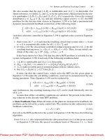
In what follows, we present solutions to the problem without detailed proofs. We
start first with the simplest case, when the given system
satisfies the following
assumptions of the so-called regular case:
1.
P
has no invariant zeros on the imaginary axis and is of maximal column
rank.
2.
Q
has no invariant zeros on the imaginary axis and is of maximal row rank.
The problem is called the singular case if
does not satisfy these conditions.
The solution to the regular case of the
optimal control problem is very simple.
The optimal controller is given by (see, e.g., [91]),
(3.62)
Please purchase PDF Split-Merge on www.verypdf.com to remove this watermark.
3.4 Optimal Control 53
where
(3.63)
(3.64)
and where
and are, respectively, the stabilizing solutions
of the following Riccati equations:
(3.65)
(3.66)

Moreover, the optimal value
can be computed as follows:
trace trace (3.67)
We note that if all the states of
are available for feedback, then the optimal con-
troller is reduced to a static law
with being given as in Equation 3.63.
Next, we present two methods that solve the singular
optimal control prob-
lem. As a matter of fact, in the singular case, it is in general infeasible to obtain
an optimal controller, although it is possible under certain restricted conditions (see,
e.g., [90, 92]). The solutions to the singular case are generally suboptimal, and usu-
ally parameterized by a certain tuning parameter, say
. A controller parameterized
by
is said to be suboptimal if there exists an such that for all
the closed-loop system comprising the given plant and the controller is asymptoti-
cally stable, and the resulting closed-loop transfer function from
to , which is
obviously a function of
, has an -norm arbitrarily close to as tends to .
The following is a so-called perturbation approach (see, e.g., [93]) that would
yield a suboptimal controller for the general singular case. We note that such an
approach is numerically unstable. The problem becomes very serious when the given
system is ill-conditioned or has multiple time scales. In principle, the desired solution
can be obtained by introducing some small perturbations to the matrices
, ,
and , i.e.
(3.68)
and

(3.69)
A full-order
suboptimal output feedback controller is given by
(3.70)
where
Please purchase PDF Split-Merge on www.verypdf.com to remove this watermark.
54 3 Linear Systems and Control
(3.71)
(3.72)
and where
and are respectively the solutions of the following
Riccati equations:
(3.73)
(3.74)
Alternatively, one could solve the singular case by using numerically stable algo-
rithms (see, e.g., [90]) that are based on a careful examination of the structural prop-
erties of the given system. We separate the problem into three distinct situations:
1) the state feedback case, 2) the full-order measurement feedback case, and 3) the
reduced-order measurement feedback case. The software realization of these algo-
rithms in MATLAB
R
can be found in [53]. For simplicity, we assume throughout the
rest of this subsection that both subsystems
P
and
Q
have no invariant zeros on the
imaginary axis. We believe that such a condition is always satisfied for most HDD
servo systems. However, most servo systems can be represented as certain chains of
integrators and thus could not be formulated as a regular problem without adding

dummy terms. Nevertheless, interested readers are referred to the monograph [90]
for the complete treatment of
optimal control using the approach given below.
i. State Feedback Case. For the case when
in the given system of Equation
3.48, i.e. all the state variables of
are available for feedback, we have the following
step-by-step algorithm that constructs an
suboptimal static feedback control law
for .
S
TEP
3.4.
C
.
S
.1: transform the system
P
into the special coordinate basis as given
by Theorem 3.1. To all submatrices and transformations in the special coordinate
basis of
P
, we append the subscript
P
to signify their relation to the system
P
.
We also choose the output transformation
P
to have the following form:

P
P
P
(3.75)
where
P
rank . Next, define
P
P
P
P
P
P
P
P
P
P
P
(3.76)
P P
P
P P
P
P
(3.77)
P P P
P
P
P
P

(3.78)
P
P
P
P
P
P
P
P
(3.79)
P
P
P
P
P
P
P
P
P
P
(3.80)
Please purchase PDF Split-Merge on www.verypdf.com to remove this watermark.