Tài liệu Phân tích tín hiệu P5 docx
Bạn đang xem bản rút gọn của tài liệu. Xem và tải ngay bản đầy đủ của tài liệu tại đây (1.19 MB, 42 trang )
Signal Analysis: Wavelets,Filter Banks, Time-Frequency Transforms and
Applications. Alfred Mertins
Copyright 0 1999 John Wiley & Sons Ltd
Print ISBN 0-471-98626-7 Electronic ISBN 0-470-84183-4
Chapter 5
Transforms and Filters
for Stochastic Processes
In this chapter, we consider the optimal processing of random signals. We
start with transforms that have optimal approximation properties,
in the
least-squares sense, for continuous and discrete-time signals, respectively.
Then we discuss the relationships between discrete transforms, optimal linear
estimators, and optimal linear filters.
5.1
The Continuous-Time Karhunen-Lo'eve
Transform
Among all linear transforms, the Karhunen-Lo bve transform (KLT) is the
one which best approximates a stochastic process in the least squares sense.
Furthermore, the KLT is a signal expansion with uncorrelated coefficients.
These properties make it interesting for many signal processing applications
such as coding and pattern recognition. The transform can be formulated for
continuous-time and discrete-time processes. In this section, we sketch the
continuous-time case [81], [l49 ].The discrete-time case will be discussed in
the next section in greater detail.
Consider a real-valued continuous-time random process z ( t ) , a
101
< t < b.
102
Chapter 5. Transforms Processes
Filters
and
Stochastic
for
We may not assume that every sample function of the random process lies in
Lz(a,b) and can be represented exactly via a series expansion. Therefore, a
weaker condition is formulated, which states that we are looking for a series
expansion that represents the stochastic process in the mean:’
N
The “unknown” orthonormal basis {vi@); i = 1 , 2 , . . .} has to be derived
from the properties of the stochastic process. For this, we require that the
coefficients
= (z, =
Pi)
2
i
l
b
Z(t)
Pi(t) dt
(5.2)
of the series expansion are uncorrelated. This can be expressed as
!
=
xj &j.
The kernel of the integralrepresentationin(5.3)
function
T,,(t,
U)
= E { 4 t ) 4)
.)
is the autocorrelation
(5.4)
*
We see that (5.3) is satisfied if
Comparing (5.5) with the orthonormality relation
realize that
ll.i.m=limit in the mean[38].
Sij
= S cpi(t)c p j ( t ) dt, we
,
b
103
5.2. The Discrete Karhunen-Lobe
Transform
must hold in order to satisfy (5.5). Thus, the solutions c p j ( t ) , j = 1 , 2 , .. .
of theintegralequation
(5.6) form the desired orthonormal basis. These
functions are also called eigenfunctions of the integral operator in (5.6). The
values X j , j = 1 , 2 , .. . are the eigenvalues. If the kernel ~,,(t,U ) is positive
definite, that is, if SJT,,(~,U)Z(~)Z(U) > 0 for all ~ ( t )La(a,b),then
d t du
E
the eigenfunctions form a complete orthonormal basis for L ~ ( u , Further
b).
properties and particular solutions of the integral equation are for instance
discussed in [149].
Signals can be approximated by carrying out the summation in (5.1) only
for i = 1 , 2 , .. . , M with finite M . The mean approximation error produced
thereby is the sumof those eigenvalues X j whose corresponding eigenfunctions
are not used for the representation. Thus, we obtain an approximation with
minimal mean square error if those eigenfunctions are used which correspond
to the largest eigenvalues.
Inpractice, solving anintegralequation
represents a majorproblem.
Therefore the continuous-time KLT is of minor interest with regard to practical applications. However, theoretically, that is, without solving the integral
equation,thistransform is an enormous help. We can describe stochastic
processes by means of uncorrelated coefficients, solveestimation orrecognition
problems for vectors with uncorrelated components and then interpret the
results for the continuous-time case.
5.2
The DiscreteKarhunen-LoheTransform
We consider a real-valued zero-mean random process
X =
[?l,
XEIR,.
Xn
The restriction to zero-mean processes means no loss of generality, since any
process 2: with mean m, can be translated into a zero-mean process X by
x=z-m2.
(5.8)
With an orthonormal basis U = ( ~ 1 , .. . , U,}, the process can be written
as
x=ua,
(5.9)
where the representation
a = [ a l , .. . ,a,] T
(5.10)
104
Chapter 5. Tkansforms and Filters Processes
Stochastic
for
is given by
a = uT X.
(5.11)
As for the continuous-time case, we derive the KLT by demanding uncorrelated coefficients:
E {aiaj} = X j
i , j = 1 , . . . ,n.
Sij,
(5.12)
The scalars X j , j = 1 , . . . ,n are unknown real numbers with X j 2 0. From
(5.9) and (5.12) we obtain
E {urx x T u j } = X j
i , j = 1 , . . . , n.
Sij,
(5.13)
Wit h
R,, = E
(5.14)
{.X.'}
this can be written as
UT R,,
u =Xj
j
Si, ,
i, j = 1 , . . . ,n.
(5.15)
We observe that because of uTuj = S i j , equation (5.15) is satisfied if the
vectors u , = 1, . . . ,n are solutions to the eigenvalue problem
j j
R,,
u = Xjuj,
j
j = 1 , . . . ,n.
(5.16)
Since R,, is a covariance matrix, the eigenvalue problem has the following
properties:
1. Only real eigenvalues X i exist.
2. A covariance matrix is positive definite or positive semidefinite, that is,
for all eigenvalues we have Xi 2 0.
3. Eigenvectors that belong to different eigenvalues are orthogonal to one
another.
4. If multiple eigenvalues occur, their eigenvectors are linearly independent
and can be chosen to be orthogonal to one another.
Thus, we see that n orthogonal eigenvectors always exist. By normalizing
the eigenvectors, we obtain the orthonormal basis of the Karhunen-LoBve
transform.
Complex-Valued Processes.
condition (5.12) becomes
For
complex-valued
processes
X
E
(En7
105
5.2. The Discrete Karhunen-Lobe Transform
This yields the eigenvalue problem
R,,
uj
= X j u j , j = 1 , . . . ,n
with the covariance matrix
R,, = E {zz"} .
Again, the eigenvalues are real and non-negative. The eigenvectors are orthogonal to one another such that U = [ u l , . . ,U,] is unitary.
From the uncorrelatedness of the complex coefficients we cannot conclude that their real andimaginary partsare also uncorrelated; that is,
E {!J%{ai} { a j } }= 0, i, j = 1,. . . ,n is not implied.
9
Best Approximation Property of the KLT. We henceforth assume that
the eigenvalues are sorted such that X 1 2 . . . 2 X From (5.12) we get for
,
.
the variances of the coefficients:
E { Jail2} x i ,
=
i = 1 , ...,R..
(5.17)
For the mean-square error of an approximation
m
D=
Cai
ui,
m
< n,
(5.18)
i=l
we obtain
(5.19)
=
5 xi.
i=m+l
It becomes obvious that an approximation
with thoseeigenvectors u1,. . . , um,
which belong to the largest eigenvectors leads to a minimal error.
In order to show that the KLT indeed yields the smallest possible error
among all orthonormal linear transforms, we look at the maximization of
C z l E { J a i l }under the condition J J u i=J1. With ai = U ~ this means
J
Z
106
Chapter 5. Tkansforms and Filters for Stochastic Processes
Figure 5.1. Contour lines of the pdf of a process z = [zl,
zZIT.
where y are Lagrange multipliers. Setting the gradient to zero yields
i
R X X U i
= yiui,
(5.21)
which is nothing but the eigenvalue problem (5.16) with y = Xi.
i
Figure 5.1 gives a geometric interpretation of the properties of the KLT.
We see that u1 points towards the largest deviation from the center of gravity
m.
Minimal Geometric Mean Property of the KLT. For any positive
definite matrix X = X i j , i, j = 1, . . . ,n the following inequality holds [7]:
(5.22)
Equality is given if X is diagonal. Since the KLT leads to a diagonal
covariance matrix of the representation, this means that the KLT leads to
random variables with a minimal geometric mean of the variances. From this,
again, optimal properties in signal coding can be concluded [76].
The KLT of White Noise Processes. For the special case that R,, is
the covariance matrix of a white noise process with
R,, = o2 I
we have
X1=X2=
...= X n = 0 2 .
Thus, the KLT is not unique in this case. Equation (5.19) shows that a white
noise process can be optimally approximated with any orthonormal basis.
107
5.2. The Discrete Karhunen-Lobe
Transform
Relationships between Covariance Matrices. In the following we will
briefly list some relationships between covariance matrices. With
A=E{aaH}=
[
A1
...
01,
(5.23)
we can write (5.15) as
A = UHR,,U.
(5.24)
Observing U H = U-', We obtain
R,, = U A U H .
(5.25)
Assuming that all eigenvalues are larger than zero, A-1 is given by
Finally, for R;: we obtain
R;: = U K I U H .
(5.27)
Application Example. In pattern recognition it is important to classify
signals by means of a fewconcise features. The signals considered in this
example aretakenfrom
inductive loops embedded in the pavement of a
highway in order to measure the change of inductivity while vehicles pass over
them. The goal is to discriminate different types of vehicle (car, truck, bus,
etc.). In the following, we will consider the two groups car and truck. After
appropriate pre-processing (normalization of speed, length, and amplitude)
we
obtain the measured signals shown in Figure 5.2, which are typical examples
of the two classes. The stochastic processes considered are z1 (car) and z2
(truck). The realizations are denoted as izl, i z ~ i,= 1 . . . N .
In a first step, zero-mean processes are generated:
(5.28)
The mean values can be estimated by
.
N
(5.29)
108
Chapter 5. Tkansforms and Filters for Stochastic Processes
1
0.8
t
0.6
8 0.4
0.2
'0
0.2
0.4
0.6
0.8
1
1
0.8
1 0.6
0.6
8 0.4
c 0.4
0.2
0
- Original
- Original
.. .. . .. Approximation
0.2
0.4
0.6
. .. .. . . Approximation
0.2
0.8
1
'0
0.2
0.4
0.6
t -
1
0.8
t+
Figure 5.2. Examples of sample functions; (a) typical signal contours; (b) two
sample functions and their approximations.
and
-
N
(5.30)
Observing the a priori probabilities of the two classes, p1 and p 2 , a process
2
=PlZl+
(5.31)
P222
can be defined. The covariance matrix R,, can be estimated as
N
R,, = E { x x ~ M
}
C
N+1,
P1
-
N
ixl
ixT
a= 1
P2
+ -C
N+1, 1
a=
ix2 ix;,
(5.32)
where i x l and ix2 are realizations of the zero-mean processes x1 and
respectively.
The first ten eigenvalues computed from a training set are:
X1
X2
X3
X5
X4
X6
X7
X8
X9
22,
X10
968 2551 3139
We see that by using only a few eigenvectors a good approximation can
be expected. To give an example,Figure 5.2 shows two signals andtheir
109
5.3. The KLT of Real-Valued AR(1) Processes
approximations
(5.33)
with the basis
{ul,u2,u3,~4}.
In general, the optimality andusefulness of extracted featuresfor discrimination is highly dependent on the algorithm that is used to carry out the
discrimination. Thus, the feature extraction method
described in this example
is not meant to be optimal for all applications. However, it shows how a high
proportion of information about a process can be stored within a features.
few
For more details on
classification algorithms and further transforms feature
for
extraction, see [59, 44, 167, 581.
5.3
The KLT of Real-Valued AR(1) Processes
An autoregressiwe process of order p (AR(p) process) is generated by exciting
a recursive filter of order p with a zero-mean, stationary white noise process.
The filter has the system function
1
H ( z )=
c p ( i ) z-i
P
1-
P ( P ) # 0.
>
(5.34)
i=l
Thus, an AR(p) process )
.
(
X
is described by the difference equation
V
+ C p ( i ) X.
(
= W(.)
)
.
(
X
- i),
(5.35)
i=l
where W(.)
is white noise. The AR(1) process with difference equation
)
.
(
X
= W(.)
+p X
(
.
- 1)
(5.36)
is often used as a simple model. It is also known as a first-order Markow
process. From (5.36) we obtain by recursion:
)
.
(
X
=c p i
W(.
- i).
(5.37)
i=O
For determining the variance of the process X
(
.
)
,
mw = E { w ( n ) }= 0
+
we use the properties
m, = E { z ( n ) }= 0
(5.38)
110
Chapter 5. Tkansforms and Filters Processes
Stochastic
for
and
?-,,(m)
= E {w(n)w(n
+ m)} = 02smo,
where SmO is the Kronecker delta. Supposing IpI
(5.39)
< 1, we get
i=O
-
U2
1- p2’
For the autocorrelation sequence we obtain
i=O
We see thatthe autocorrelationsequence is infinitely long. However,
henceforth only the values rzz(-N l),.... T,,(N - 1) shall be considered.
Because of the stationarity of the input process, the covariance matrix of the
AR(1) process is a Toeplitz matrix. It is given by
+
o2
R,, = -
(5.42)
1 - p2
The eigenvectors of R,, form the basis of the KLT. For real signals and
even N , the eigenvalues Xk, Ic = 0,. ... N - 1 and the eigenvectors were
analytically derived by Ray and Driver [123]. The eigenvalues are
1
Xk
=
I
1- 2 p cos(ak)
+ p2 ’
k=O,
.... N - 1 ,
(5.43)
111
5.4. Whitening Transforms
where
ak,
5 = 0 , . . . ,N
- 1 denotes
tan(Nak) = -
the real positive roots of
(1 - p’) sin(ak)
cos(ak) - 2p p COS(Qk).
+
(5.44)
The components of the eigenvectors u k , k = 0 , . . . ,N - 1 are given by
5.4
Whitening Transforms
In this section we are concerned with the problem of transforming a colored
noise process into a white noise process. That is, the coefficients of the
representation should not only be uncorrelated (as for the KLT), they should
also have the same variance. Such transforms, known as whitening transforms,
are mainly applied in signal detection and pattern recognition, because they
lead t o a convenient process representation with additive white noise.
Let n be a process with covariance matrix
Rnn = E { n n H }
#
a21.
(5.46)
We wish t o find a linear transform T which yields an equivalent process
ii=Tn
(5.47)
wit h
E
{iiiiH}
= E { T n n H T H= TR,,TH = I .
}
(5.48)
We already see that the transform cannot be unique since by multiplying an
already computed matrix T with an arbitrary unitary matrix,
property (5.48)
is preserved.
The covariance matrix can be decomposed as follows (KLT):
R,, = U A U H = U X E H U H .
For A and X we have
(5.49)
Chapter 5. Tkansforms and Filters Processes
Stochastic
for
112
Possible transforms are
T = zP1UH
(5.50)
T =U T I U H .
(5.51)
or
This can easily be verified by substituting (5.50) into (5.48):
(5.52)
Alternatively, we can apply the Cholesky decomposition
R,, = L L H ,
(5.53)
where L is a lower triangular matrix. The whitening transform is
T = L-l.
(5.54)
For the covariance matrix we again have
E
{+inH)T R , , T ~= L - ~ L L H L H - '= I .
=
(5.55)
In signal analysis, one often encounters signals of the form
r=s+n,
(5.56)
where S is a known signal and n is an additive colored noise processes. The
whitening transforms transfer (5.56) into an equivalent model
F=I+k
(5.57)
with
F
= Tr,
(5.58)
I = Ts,
ii
= Tn,
where n is a white noise process of variance
IS:1.
=
113
5.5. Linear Estimation
5.5
Linear Estimation
Inestimationthe
goal is to determine a set of parametersas precisely
as possible from noisy observations. Wewill focus on the case where the
estimators are linear, that is, the estimates for the parameters are computed
as linear combinations of the observations. This problem is closely related to
the problem of computing the coefficients of a series expansion of a signal, as
described in Chapter 3.
Linear methods do not require precise knowledge of the noise statistics;
only moments up to the second order are taken into account. Therefore they
are optimal only under the linearity constraint, and, in general, non-linear
estimators with better properties may be found. However, linear estimators
constitutethe globally optimal solution as far as Gaussian processes are
concerned [ 1491.
5.5.1
Least-Squares Estimation
We consider the model
r=Sa+n,
(5.59)
where r is our observation, a is the parameter vector in question, and n is a
noise process. Matrix S can be understood as a basis matrix that relates the
parameters to the clean observation S a .
The requirement to have an unbiased estimate can be written as
E { u ( r ) l a }= a,
(5.60)
where a is understood as an arbitrarynon-random parameter vector. Because
of the additive noise, the estimates u ( r ) l aagain form a random process.
The linear estimation approach is given by
h(.) = A r .
(5.61)
If we assume zero-mean noise n , matrix A must satisfy
A S = I
(5.62)
114
Chapter 5. Tkansforms and Filters Processes
Stochastic
for
in order to ensure unbiased estimates. This is seen from
E{h(r)la} = E { A rla}
= A E{rla}
= AE{Sa+n}
=
(5.63)
A S a
The generalized least-squares estimator is derived from the criterion
!
.
= mm,
(5.64)
CY = &(r)
where an arbitrary weighting matrix G may be involved in the definition of
the inner product that induces the norm in (5.64). Here the observation r is
considered as a single realization of the stochastic process r . Making use of
the fact that orthogonal projections yield a minimal approximation error,we
get
a(r) = [SHGS]-lSHGr
(5.65)
according to (3.95). Assuming that [SHGS]-l
exists, the requirement (5.65)
to have an unbiased estimator is satisfied for arbitrary weighting matrices, as
can easily be verified.
If we choose G = I , we speak of a least-squares estimator. For weighting
matrices G # I , we speak of a generalized least-squares estimator. However,
the approach leaves open the question of how a suitable G is found.
5.5.2
The Best Linear Unbiased Estimator (BLUE)
As will be shown below, choosing G = R;:, where
R,, = E { n n H }
(5.66)
is the correlation matrix of the noise, yields an unbiased estimatorwith
minimal variance. The estimator, which is known as the best linear unbiased
estimator (BLUE), then is
A = [SHR;AS]-'SHR;A.
(5.67)
The estimate is given by
u ( r )=
[s~R;AsS]-~S~R;A
r.
(5.68)
115
5.5. Linear Estimation
The variances of the individual estimates can be found on the main diagonal
of the covariance matrix of the error e = u ( r )- a, given by
R,, = [SHRiAS]-'.
Proof of (5.69) and theoptimality
AS = I we have
h ( r )--la
(5.69)
of (5.67). First, observe that with
=
A S a+A n-a
=
An.
(5.70)
Thus,
R,,
=
AE { n n H } A H
=
AR,,A~
=
[SHR;AS]-'SHR;ARn,R;AS[SHR;AS]-'
=
[SHR;AS]-'.
(5.71)
In order to see whether A according to (5.67) is optimal, an estimation
(5.72)
with
(5.73)
will be considered. The urlbiasedness constraint requires that
As==.
(5.74)
Because of A S = I this means
DS=O
(null matrix).
(5.75)
For the covariance matrix of the error E(r) = C(r)- a we obtain
=
AR,,A-H
=
[ A D]Rnn[A DIH
+
+
+ ARnnDH+ DRnnAH+ DRnnDH.
= ARnnAH
(5.76)
116
Chapter 5. Tkansforms and Filters for Stochastic Processes
With
(AR,nDH)H DRn,AH
=
= DRnnR$S[SHRiAS]-'
=
DSISHR;AS]-l
v
0
(5.77)
= o
(5.76) reduces to
R 2 = ARn,AH + DRnnDH.
2
(5.78)
We see that Rc2 is the sum of two non-negative definite expressions so that
minimal main diagonal elementsof Rgc are yielded for D = 0 and thus for A
according to (5.67). 0
In the case of a white noise process n , (5.68) reduces to
S(r) = [
s~s]-~s~~.
(5.79)
Otherwise the weighting with G = R;; can be interpreted as an
implicit
whitening of the noise. This can beseen by using the Cholesky decomposition
R,, = LLH and and by rewriting the model as
F=Sa+fi,
where
F
= L-'r,
(5.80)
3 = L - ~ s ,fi = L-ln.
(5.81)
The transformedprocess n is a white noise process. The equivalent estimator
then is
- HH
- U(?) = [ S ~ 1 - l r ~
.
(5.82)
I
5.5.3
MinimumMeanSquareError
Estimation
The advantage of the linear estimators considered in the previous section
is their unbiasedness. If we dispensewith this property,estimateswith
smaller mean square error may
be found. Wewill start the discussion on
the assumptions
E { r } = 0,
E { a } = 0.
(5.83)
Again, the linear estimator is described by a matrix A:
S(r) = A r .
(5.84)
117
5.5. Linear Estimation
Here, r is somehow dependent on a , but the inner relationship between r
and a need not be known however. The matrix A which yields minimal main
diagonal elements of the correlation matrix of the estimation error e = a - U
is called the minimum mean square error (MMSE) estimator.
In order to find the optimal A , observe that
{
=
E [ U - U ] [U - U ]
=
R,,
E{aaH}-E{UaH}-E{aUH}+E{UUH}.
(5.85)
Substituting (5.84) into (5.85) yields
R,, = R,, - AR,, - R,,AH + AR,,AH
(5.86)
with
R,,
=
E {aaH},
R,,
=
R: = E { r a H } ,
R,,
= E{mH}.
(5.87)
Assuming the existence of R;:, (5.86) can be extended by
R,, R;: R,,
- R,, R;:
R,,
and be re-written as
R,, = [ A - R,,RF:] R,, [AH- RF:Ra,]
-
RTaRF:Ra,+ Raa.(5.88)
Clearly, R,, has positive diagonal elements. Since only the first term on the
right-hand side of (5.88) is dependenton A , we have a minimum of the
diagonal elements of R,, for
A = R,, R;:.
(5.89)
The correlation matrix of the estimation error is then given by
Re,
= R a a - RTaR;:RaT*
(5.90)
Orthogonality Principle. In Chapter 3 we saw that approximations D of
signals z are obtained with minimal error if the error D - z is orthogonal to
D. A similar relationship holds between parameter vectors a and their MMSE
estimates. With A according to (5.89) we have
R,, = A R,,,
i.e.
E { a r H }= A E { r r H }.
(5.91)
118
Chapter 5. Tkansforms
Filters
and
Stochastic
for Processes
This means that the following orthogonality relations hold:
E [S - a] SH
{
}
- R&,
=
=
[AR,, - R,,] A"
=
0.
(5.92)
With A r = S the right part of (5.91) can also be written as
E { a r H } E {Sr"} ,
=
(5.93)
E { [ S - a] r H }= 0.
(5.94)
which yields
The relationship expressed in (5.94) is referred to as the orthogonality
principle. The orthogonality principle states that we get an MMSE estimate
if the error S(r)- a is uncorrelated to all components of the input vector r
used for computing S ( r ) .
Singular Correlation Matrix. There
are cases where the correlation
matrix R,, becomes singular and the linear estimator cannot be written as
A = R,, R;:.
(5.95)
A more general solution, which involves the replacement of the inverse by the
pseudoinverse, is
A = R,, R:,.
(5.96)
In order to show the optimality of (5.96), the estimator
A=A+D
(5.97)
with A according to (5.96) and an arbitrary matrix D is considered. Using
the properties of the pseudoinverse, we derive from (5.97) and (5.86):
R,,
- H
- H
= R,, - AR,, - R,,A
= R,, - R,,R:,R,,
+ AR,,A
+DR:,D~.
(5.98)
Since R:, is at least positive semidefinite, we get a minimum of the diagonal
elements of R,, for D = 0, and (5.96) constitutes oneof the optimalsolutions.
Additive Uncorrelated Noise. So far, nothing has been about possible
said
dependencies between a and the noise contained in r . Assuming that
r=Sa+n,
(5.99)
119
5.5. Linear Estimation
where n is an additive, uncorrelated noise process, we have
(5.100)
and A according to (5.89) becomes
A = R,,SH
[SR,,SH
+ R,,]-1.
(5.101)
Alternatively, A can be written as
1
+ SHRLAS]- SHRLA.
A = [R;:
(5.102)
This is
verified
by
equating (5.101) and (5.102), and by multiplying the
obtained expression with [R;: +SHR;AS]from the left and with [SR,,SH+
R,,] from the right, respectively:
[R;:
+ SHRLAS]R,,SH = SHRLA[SR,,SH R , , ] .
+
The equality of both sides is easily seen. The matrices to inverted in (5.102),
be
except R,,, typically have a much smaller dimension than those in (5.101). If
the noise is white, R;; can be immediately
stated, and(5.102) is advantageous
in terms of computational cost.
For R,, we get from (5.89), (5.90), (5.100) and (5.102):
Ree
= Raa - ARar
= R,, - [R;;
Multiplying (5.103) with [R;;
+ S H R ; ; S ] - ~SHR;;SR,,.
(5.103)
+ SHR;;S] from the left yields
= I,
(5.104)
so that the following expression is finally obtained:
+
Re, = [R,-,' S H R i A S ] - l .
(5.105)
Equivalent Estimation Problems. We partition A and a into
(5.106)
120
Chapter 5. Tkansforms
Filters
and
Stochastic
for Processes
such that
(5.107)
If we assume that the processes a l , a2 and n are independent of one another,
the covariance matrix R,, and its inverse R;: have the form
and A according to (5.102) can be written as
where S = [SI,5'21. Applying the matrix equation
€
3
€-l
+E-132)-1BE-1
4 - 1 3 2 ) - 1
2)-l
2)
(5.110)
= 3c - &?€-l3
yields
with
Rn1n1
+ SzRazazSf,
Rnn + S1Ra1a1Sf.
= Rnn
(5.113)
=
(5.114)
The inverses R;:nl and R;inz can be written as
=
R;:nz
[R;:
=
[R;: -
- RiiS2
(SfRiAS2
+ R;:az)-1 SfRiA] ,(5.115)
+
(SyR;AS1 R;:al)- 1 SyR;:] .(5.116)
Equations (5.111) and (5.112) describe estimations of a1 and a in the
2
models
r = S l a l + nl,
(5.117)
121
5.5. Linear Estimation
r = S2a2
+n2
(5.118)
with
(5.119)
Thus, each parameter to be estimated can be understood as noise in the
estimation of the remaining parameters.An exception is given if SFR$S2 =
0 , which means that S1 and S2 are orthogonal to each other with respect to
the weighting matrix R;:. Then we get
and
Re,,, = [SBRLASI+
and we observe that the second signal component Sza2 has no influence on
the estimate.
Nonzero-Mean Processes. One could imagine that the precision of linear
estimations with respect to nonzero-mean processes r and a can be increased
compared to thesolutions above if an additional term taking care the mean
of
values of the processes is considered. In order to describe this more general
case, let us denote the mean of the parameters as
=E{a}.
(5.120)
The estimate is now written as
iL=Ar+c%+c,
(5.121)
where c is yet unknown. Using the shorthand
b = a--,
b = h--,
M
=
[c,A]
(5.122)
(5.121) can be rewritten as:
b =Mx.
(5.123)
122
Chapter 5. Tkansforms
Filters
and
Stochastic
for Processes
The relationship between b and X is linear as usual, so that the optimal M
can be given according to (5.89):
M = R,bR$.
(5.124)
Now let us express R , b and R;: through correlation matrices of the processes
a and T . From (5.122) and E { b } = 0 we derive
(5.125)
with
R,b
= E{[U
-
si]
= E{[a-si]
T"}
(5.126)
[T-e]"},
where
F=E{r}.
(5.127)
R,, writes
1
= [F
FH
(5.128)
RT,]'
Using (5.110) we obtain
R;: =
1
+ e"
[R,, - ee"] - l
e
- [R,, - ee"1-l e
-e" [R,, - FP"]
-l
[R,, - FP"]
-l
(5.129)
From (5.122) - (5.129) and
[R,, - Fe"] = E { [T - e] [T - e]"}
(5.130)
we finally conclude
U = E { [a- s i ]
[T
- e]"}
E { [T - e] [T - e]"}-l
[T
-
e] + a.
(5.131)
Equation (5.131) can be interpreted as
follows: the nonzero-mean processes
a and r are first modified so as to become zero-mean processes a - si and
r - e. For the zero-mean processes the estimation problem can be solved as
usual. Subsequently the mean value si is added in order to obtain the final
estimate U.
Unbiasedness for Random Parameter Vectors. So far the parameter
vector to be estimated was assumed to be non-random. If we consider a to
be a random process, various other weaker definitions of unbiasedness are
possible.
123
5.5. Linear Estimation
The straightforward requirement
is meaningless, because it satisfied for any A as faras r and a are zero-mean.
is
A useful definition of unbiasedness in the case of random parameters is to
consider one of the parameters contained in a (e.g. a k ) as non-random and to
regard all other parameters a l , . . . , ak-1, ak+l etc. as random variables:
In order to obtain an estimator which is unbiased in the sense of (5.133), the
equivalences discussed above may be applied. Starting with the model
=
Sa+n
=
r
skak
(5.134)
+n ,
in which n contains the additive noise n and the signal component produced
by all random parameters a j , j # k, we can write the unbiased estimate as
H
6, = h, r
(5.135)
A = [hl,h z , .. .IH
(5.137)
Then,
is an estimator which is unbiased in the sense of (5.133).
The Relationship between MMSE Estimation and the BLUE. I
f
R,, = E { a a H }is unknown, R;: = 0 is substituted into (5.102), and we
obtain the BLUE (cf. (5.67)):
A = [SHRiAS]-l
SHRP1
nn
(5.138)
In the previous discussion it became obvious that it is possible to obtain
unbiased estimates of some of the parameters and to estimate the others
withminimummeansquareerror.This
result is of special interest if no
unbiased estimator can be stated
for all parameters because of a singular
matrix SHR;AS.
124
Chapter 5. Tkansforms and Filters Processes
Stochastic
for
5.6
Linear
Optimal
5.6.1
Filters
Wiener Filters
We consider the problem depictedin Figure 5.3. By linear filtering of the noisy
signal r ( n ) = z(n) w ( n ) we wish to make y(n) = r ( n ) * h(n) as similar as
possible to a desired signal d ( n ) . The quality criterion used for designing the
optimal causal linear filter h(n)is
+
The solution to this optimization problem can easily be stated by applying
the orthogonalityprinciple. Assuming a causal FIR filter h(n) of length p , we
have
c
P-1
y(n) =
h(i)r ( n - i).
(5.140)
i=O
Thus, according to (5.94), the following orthogonality condition mustbe
satisfied by the optimal filter:
For stationary processes r ( n ) and d ( n ) this yields the discrete form of the
so-called Wiener-Hopf equation:
c
P-1
j = 0, 1 , . . . , p - 1,
(5.142)
h(i) r,,(j - i) = TT&),
i=O
with
(5.143)
The optimal filter is found by solving (5.142).
An applicationexample is theestimation of data d(n) from a noisy
observation r ( n ) = Cec(C) d ( n - l ) w(n), where)(
.C
is a channel and
W.
(
)
is noise. By using the optimal filter h(n) designed according to (5.142)
the data is recovered with minimal mean square error.
+
5.6. Linear Optimal Filters
1
125
'
\ ,
I
44
Noise
w(n)
Figure 5.3. Designing linear optimal filters.
Variance. For the variance of the error we have
w- 1
w- 1
(5.144)
i=O
i=O
with 0 = E { ld(n12}. Substituting the optimal solution (5.142) into (5.144)
:
yields
P-1
(5.145)
Matrix Notation. In matrix notation (5.142) is
(5.146)
wit h
(5.147)
(5.148)
and