Tài liệu Modeling Of Data part 7 pptx

15.6 Confidence Limits on Estimated Model Parameters
689
Sample page from NUMERICAL RECIPES IN C: THE ART OF SCIENTIFIC COMPUTING (ISBN 0-521-43108-5)
Copyright (C) 1988-1992 by Cambridge University Press.Programs Copyright (C) 1988-1992 by Numerical Recipes Software.
Permission is granted for internet users to make one paper copy for their own personal use. Further reproduction, or any copying of machine-
readable files (including this one) to any servercomputer, is strictly prohibited. To order Numerical Recipes books,diskettes, or CDROMs
visit website or call 1-800-872-7423 (North America only),or send email to (outside North America).
15.6 Confidence Limits on Estimated Model
Parameters
Several times alreadyinthischapter wehave made statementsaboutthestandard
errors, or uncertainties, in a set of M estimated parameters a. We have given some
formulas for computing standard deviations or variances of individual parameters
(equations 15.2.9, 15.4.15, 15.4.19), as well as some formulas for covariances
between pairs of parameters (equation 15.2.10; remark following equation 15.4.15;
equation 15.4.20; equation 15.5.15).
In this section, we want to be more explicit regarding the precise meaning
of these quantitative uncertainties, and to give further information about how
quantitative confidence limits on fitted parameters can be estimated. The subject
can get somewhat technical, and even somewhat confusing, so we will try to make
precise statements, even when they must be offered without proof.
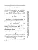
Figure 15.6.1 shows the conceptual scheme of an experiment that “measures”
a set of parameters. There is some underlying true set of parameters a
true
that are
known to Mother Nature but hidden from the experimenter. These true parameters
are statistically realized, along with random measurement errors, as a measured data
set, which we will symbolizeasD
(0)
. Thedataset D
(0)
isknown to the experimenter.

He or she fits the data to a model by χ
2
minimization or some other technique, and
obtains measured, i.e., fitted, values for the parameters, which we here denote a
(0)
.
Because measurement errors have a random component, D
(0)
is not a unique
realization of the true parameters a
true
. Rather, there are infinitely many other
realizations of the true parameters as “hypothetical data sets” each of which could
have been the one measured, but happened not to be. Let us symbolize these
by D
(1)
,D
(2)
,.... Each one, had it been realized, would have given a slightly
different set of fitted parameters, a
(1)
, a
(2)
,..., respectively. These parameter sets
a
(i)
therefore occur with some probability distribution in the M-dimensional space
of all possible parameter sets a. The actual measured set a
(0)
is one member drawn

from this distribution.
Even more interesting than the probability distribution of a
(i)
would be the
distribution of the difference a
(i)
− a
true
. This distribution differs from the former
one by a translation that puts MotherNature’s true value at the origin. If we knew this
distribution, we would know everything that there is to know about the quantitative
uncertainties in our experimental measurement a
(0)
.
So the name of the game is to find some way of estimating or approximating
the probability distributionof a
(i)
−a
true
without knowing a
true
and withouthaving
available to us an infinite universe of hypothetical data sets.
Monte Carlo Simulation of Synthetic Data Sets
Although the measured parameter set a
(0)
is not the true one, let us consider
a fictitious world in which it was the true one. Since we hope that our measured
parameters are not too wrong, we hope that that fictitious world is not too different
from the actual world with parameters a

true
. In particular, let us hope — no, let us
assume — that the shape of the probability distribution a
(i)
− a
(0)
in the fictitious
worldis the same, or very nearly the same, as the shape of the probabilitydistribution
690
Chapter 15. Modeling of Data
Sample page from NUMERICAL RECIPES IN C: THE ART OF SCIENTIFIC COMPUTING (ISBN 0-521-43108-5)
Copyright (C) 1988-1992 by Cambridge University Press.Programs Copyright (C) 1988-1992 by Numerical Recipes Software.
Permission is granted for internet users to make one paper copy for their own personal use. Further reproduction, or any copying of machine-
readable files (including this one) to any servercomputer, is strictly prohibited. To order Numerical Recipes books,diskettes, or CDROMs
visit website or call 1-800-872-7423 (North America only),or send email to (outside North America).
actual data set

hypothetical
data set
hypothetical
data set
hypothetical
data set
a
3
a
2
a
1
fitted

parameters
a
0
χ
2
min


true parameters
a
true
experimental realization
.
.
.
.
.
.
Figure 15.6.1. A statistical universe of data sets from an underlying model. True parameters a
true
are
realized in a data set, from which fitted (observed) parameters a
0
are obtained. If the experiment were
repeated many times, new data sets and new values of the fitted parameters would be obtained.
a
(i)
− a
true
in the real world. Notice that we are not assuming that a

(0)
and a
true
are
equal; they are certainly not. We are only assuming that the way in which random
errors enter the experiment and data analysis does not vary rapidly as a function of
a
true
,sothata
(0)
can serve as a reasonable surrogate.
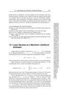
Now, often, the distribution of a
(i)
− a
(0)
in the fictitious world is within our
power to calculate (see Figure 15.6.2). If we know something about the process
that generated our data, given an assumed set of parameters a
(0)
, then we can
usually figure out how to simulate our own sets of “synthetic” realizations of these
parameters as “synthetic data sets.” The procedure is to draw random numbers from
appropriate distributions (cf. §7.2–§7.3) so as to mimic our best understanding of
the underlying process and measurement errors in our apparatus. With such random
draws, we construct data sets with exactly the same numbers of measured points,
and precisely the same values of all control (independent) variables, as our actual
data set D
(0)
. Let us call these simulated data sets D
S

(1)
,D
S
(2)
,.... By construction
these are supposed to have exactly the same statistical relationship to a
(0)
as the
D
(i)
’s have to a
true
. (For the case where you don’t know enough about what you
are measuring to do a credible job of simulating it, see below.)
Next, for each D
S
(j)
, perform exactly the same procedure for estimation of
parameters, e.g., χ
2
minimization, as was performed on the actual data to get
the parameters a
(0)
, giving simulated measured parameters a
S
(1)
, a
S
(2)
,.... Each

simulated measured parameter set yields a point a
S
(i)
− a
(0)
. Simulate enough data
sets and enoughderived simulated measured parameters, and you map out the desired
probability distribution in M dimensions.
In fact, the ability to do Monte Carlo simulations in this fashion has revo-
15.6 Confidence Limits on Estimated Model Parameters
691
Sample page from NUMERICAL RECIPES IN C: THE ART OF SCIENTIFIC COMPUTING (ISBN 0-521-43108-5)
Copyright (C) 1988-1992 by Cambridge University Press.Programs Copyright (C) 1988-1992 by Numerical Recipes Software.
Permission is granted for internet users to make one paper copy for their own personal use. Further reproduction, or any copying of machine-
readable files (including this one) to any servercomputer, is strictly prohibited. To order Numerical Recipes books,diskettes, or CDROMs
visit website or call 1-800-872-7423 (North America only),or send email to (outside North America).
synthetic
data set 1
synthetic
data set 2
synthetic
data set 3
synthetic
data set 4
a
2
χ
2

min

χ
2

min
(s)
a
1
(s)
a
3
(s)
a
4
(s)
Monte Carlo
parameters

Monte Carlo realization
fitted
parameters
a
0


actual
data set
Figure 15.6.2. MonteCarlo simulation of an experiment. The fitted parameters from an actualexperiment
are used as surrogates for the true parameters. Computer-generatedrandom numbers are used to simulate
many synthetic data sets. Each of these is analyzed to obtain its fitted parameters. The distribution of
these fitted parameters around the (known) surrogate true parameters is thus studied.

lutionized many fields of modern experimental science. Not only is one able to
characterize the errors of parameter estimation in a very precise way; one can also
try out on the computer different methods of parameter estimation, or different data
reduction techniques, and seek to minimize the uncertainty of the result according
to any desired criteria. Offered the choice between mastery of a five-foot shelf of
analytical statistics books and middling ability at performing statistical Monte Carlo
simulations, we would surely choose to have the latter skill.
Quick-and-Dirty Monte Carlo: The Bootstrap Method
Here is a powerful technique that can often be used when you don’t know
enough about the underlying process, or the nature of your measurement errors,
to do a credible Monte Carlo simulation. Suppose that your data set consists of
N independent and identically distributed (or iid) “data points.” Each data point
probably consists of several numbers, e.g., one or more control variables (uniformly
distributed, say, in the range that you have decided to measure) and one or more
associated measured values (each distributed however Mother Nature chooses).
“Iid” means that the sequential order of the data points is not of consequence to
the process that you are using to get the fitted parameters a. For example, a χ
2
sum like (15.5.5) does not care in what order the points are added. Even simpler
examples are the mean value of a measured quantity, or the mean of some function
of the measured quantities.
The bootstrap method
[1]
uses the actual data set D
S
(0)
, with its N data points, to
generate any number of synthetic data sets D
S
(1)

,D
S
(2)
,..., also with N data points.
The procedure is simply to draw N data points at a time with replacement from the
692
Chapter 15. Modeling of Data
Sample page from NUMERICAL RECIPES IN C: THE ART OF SCIENTIFIC COMPUTING (ISBN 0-521-43108-5)
Copyright (C) 1988-1992 by Cambridge University Press.Programs Copyright (C) 1988-1992 by Numerical Recipes Software.
Permission is granted for internet users to make one paper copy for their own personal use. Further reproduction, or any copying of machine-
readable files (including this one) to any servercomputer, is strictly prohibited. To order Numerical Recipes books,diskettes, or CDROMs
visit website or call 1-800-872-7423 (North America only),or send email to (outside North America).
set D
S
(0)
. Because of the replacement, you do not simply get back your original
data set each time. You get sets in which a random fraction of the original points,
typically ∼ 1/e ≈ 37%, are replaced by duplicated original points. Now, exactly
as in the previous discussion, you subject these data sets to the same estimation
procedure as was performed on the actual data, giving a set of simulated measured
parameters a
S
(1)
, a
S
(2)
,.... These will be distributed around a
(0)
in close to the same
way that a

(0)
is distributed around a
true
.
Sounds like getting something for nothing, doesn’t it? In fact, it has taken more
than a decade for the bootstrap method to become accepted by statisticians. By now,
however, enoughtheoremshave been proved to render the bootstrapreputable (see
[2]
for references). The basic idea behind the bootstrap is that the actual data set, viewed
as a probability distribution consisting of delta functions at the measured values, is
in most cases the best — or only — available estimator of the underlying probability
distribution. It takes courage, but one can often simply use that distribution as the
basis for Monte Carlo simulations.
Watch out for cases where the bootstrap’s “iid” assumption is violated. For
example, if you have made measurements at evenly spaced intervals of some control
variable, then youcan usuallygetaway withpretending that theseare “iid,” uniformly
distributed over the measured range. However, some estimators of a (e.g., ones
involving Fourier methods) might be particularly sensitive to all the points on a grid
being present. In that case, the bootstrap is going to give a wrong distribution. Also
watch out for estimators that look at anything like small-scale clumpiness within the
N data points, or estimators that sort the data and look at sequential differences.
Obviously the bootstrap will fail on these, too. (The theorems justifying the method
are still true, but some of their technical assumptions are violated by these examples.)
For a large class of problems, however, the bootstrap does yield easy, very
quick, Monte Carlo estimates of the errors in an estimated parameter set.
Confidence Limits
Rather than present all details of the probability distribution of errors in
parameter estimation, it is common practice to summarize the distribution in the
form of confidence limits. The full probability distribution is a function defined
on the M-dimensional space of parameters a.Aconfidence region (or confidence

interval) is just a region of that M-dimensional space (hopefullya small region) that
contains a certain (hopefully large) percentage of the total probability distribution.
You point to a confidence region and say, e.g., “there is a 99 percent chance that the
true parameter values fall within this region around the measured value.”
It is worth emphasizing that you, the experimenter, get to pick both the
confidence level (99 percent in the above example), and the shape of the confidence
region. The only requirement is that your region does include the stated percentage
of probability. Certain percentages are, however, customary in scientific usage:
68.3 percent (the lowest confidence worthy of quoting), 90 percent, 95.4 percent, 99
percent, and 99.73 percent. Higher confidence levels are conventionally“ninety-nine
point nine ... nine.” As for shape, obviously you want a region that is compact
and reasonably centered on your measurement a
(0)
, since the whole purpose of a
confidence limit is to inspire confidence in that measured value. In one dimension,
the convention is to use a line segment centered on the measured value; in higher
dimensions, ellipses or ellipsoids are most frequently used.
15.6 Confidence Limits on Estimated Model Parameters
693
Sample page from NUMERICAL RECIPES IN C: THE ART OF SCIENTIFIC COMPUTING (ISBN 0-521-43108-5)
Copyright (C) 1988-1992 by Cambridge University Press.Programs Copyright (C) 1988-1992 by Numerical Recipes Software.
Permission is granted for internet users to make one paper copy for their own personal use. Further reproduction, or any copying of machine-
readable files (including this one) to any servercomputer, is strictly prohibited. To order Numerical Recipes books,diskettes, or CDROMs
visit website or call 1-800-872-7423 (North America only),or send email to (outside North America).
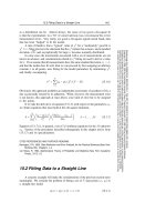
68% confidence interval on a
2
68% confidence
interval on a
1
68% confidence region

on a
1
and a
2
jointly
bias
a
(i)1
− a
(0)1
(s)
a
(i)2
− a
(0)2
(s)
Figure 15.6.3. Confidence intervals in 1 and 2 dimensions. The same fraction of measured points (here
68%) lies (i) between the two vertical lines, (ii) between the two horizontal lines, (iii) within the ellipse.
You might suspect, correctly, that the numbers 68.3 percent, 95.4 percent,
and 99.73 percent, and the use of ellipsoids, have some connection with a normal
distribution. That is true historically, but not always relevant nowadays. In general,
the probability distribution of the parameters will not be normal, and the above
numbers, used as levels of confidence, are purely matters of convention.
Figure 15.6.3 sketches a possible probability distribution for the case M =2.
Shownare threedifferent confidence regions which might usefully be given, all at the
same confidence level. The two vertical lines enclose a band (horizontal inverval)
which represents the 68 percent confidence interval for the variable a
1
withoutregard
to the value of a

2
. Similarly the horizontal lines enclose a 68 percent confidence
interval for a
2
. The ellipse shows a 68 percent confidence interval for a
1
and a
2
jointly. Notice that to enclose the same probabilityas the two bands, the ellipse must
necessarily extend outside of both of them (a point we will return to below).
Constant Chi-Square Boundaries as Confidence Limits
When the method used to estimate the parameters a
(0)
is chi-square minimiza-
tion, as in the previous sections of this chapter, then there is a natural choice for the
shape of confidence intervals, whose use is almost universal. For the observed data
set D
(0)
, the value of χ
2
is a minimum at a
(0)
. Call this minimum value χ
2
min
.If