Tài liệu Sổ tay của các mạng không dây và điện toán di động P2 pdf

CHAPTER 2
Location Management in
Cellular Networks
JINGYUAN ZHANG
Department of Computer Science, University of Alabama
2.1 INTRODUCTION
It has been known for over one hundred years that radio can be used to keep in touch with
people on the move. However, wireless communications using radio were not popular un-
til Bell Laboratories developed the cellular concept to reuse the radio frequency in the
1960s and 1970s [31]. In the past decade, cellular communications have experienced an
explosive growth due to recent technological advances in cellular networks and cellular
telephone manufacturing. It is anticipated that they will experience even more growth in
the next decade. In order to accommodate more subscribers, the size of cells must be re-
duced to make more efficient use of the limited frequency spectrum allocation. This will
add to the challenge of some fundamental issues in cellular networks. Location manage-
ment is one of the fundamental issues in cellular networks. It deals with how to track sub-
scribers on the move. The purpose of this chapter is to survey recent research on location
management in cellular networks. The rest of this chapter is organized as follows. Section
2.2 introduces cellular networks and Section 2.3 describes basic concepts of location man-
agement. Section 2.4 presents some assumptions that are commonly used to evaluate a lo-
cation management scheme in terms of network topology, call arrival probability, and mo-
bility. Section 2.5 surveys popular location management schemes. Finally, Section 2.6
summarizes the chapter.
2.2 CELLULAR NETWORKS
In a cellular network, a service coverage area is divided into smaller hexagonal areas re-
ferred to as cells. Each cell is served by a base station. The base station is fixed. It is able
to communicate with mobile stations such as cellular telephones using its radio transceiv-
er. The base station is connected to the mobile switching center (MSC) which is, in turn,
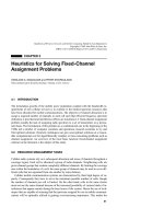
connected to the public switched telephone network (PSTN). Figure 2.1 illustrates a typi-
cal cellular network. The triangles represent base stations.
The frequency spectrum allocated to wireless communications is very limited, so the

27
Handbook of Wireless Networks and Mobile Computing, Edited by Ivan Stojmenovic´
Copyright © 2002 John Wiley & Sons, Inc.
ISBNs: 0-471-41902-8 (Paper); 0-471-22456-1 (Electronic)
cellular concept was introduced to reuse the frequency. Each cell is assigned a certain
number of channels. To avoid radio interference, the channels assigned to one cell must be
different from the channels assigned to its neighboring cells. However, the same channels
can be reused by two cells that are far apart such that the radio interference between them
is tolerable. By reducing the size of cells, the cellular network is able to increase its capac-
ity, and therefore to serve more subscribers.
For the channels assigned to a cell, some are forward (or downlink) channels that are
used to carry traffic from the base station to mobile stations, and the others are reverse (or
uplink) channels that are used to carry traffic from mobile stations to the base station.
Both forward and reverse channels are further divided into control and voice (or data)
channels. The voice channels are for actual conversations, whereas the control channels
are used to help set up conversations.
A mobile station communicates with another station, either mobile or land, via a base
station. A mobile station cannot communicate with another mobile station directly. To
make a call from a mobile station, the mobile station first needs to make a request using a
reverse control channel of the current cell. If the request is granted by the MSC, a pair of
voice channels will be assigned for the call. To route a call to a mobile station is more
complicated. The network first needs to know the MSC and the cell in which the mobile
station is currently located. How to find out the current residing cell of a mobile station is
an issue of location management. Once the MSC knows the cell of the mobile station, it
can assign a pair of voice channels in that cell for the call. If a call is in progress when the
mobile station moves into a neighboring cell, the mobile station needs to get a new pair of
voice channels in the neighboring cell from the MSC so the call can continue. This
process is called handoff (or handover). The MSC usually adopts a channel assignment
strategy that prioritizes handoff calls over new calls.
This section has briefly described some fundamental concepts about cellular networks

such as frequency reuse, channel assignment, handoff, and location management. For de-
28
LOCATION MANAGEMENT IN CELLULAR NETWORKS
Figure 2.1 A typical cellular network.
tailed information, please refer to [6, 7, 20, 31, 35]. This chapter will address recent re-
search on location management.
2.3 LOCATION MANAGEMENT
Location management deals with how to keep track of an active mobile station within the
cellular network. A mobile station is active if it is powered on. Since the exact location of
a mobile station must be known to the network during a call, location management usual-
ly means how to track an active mobile station between two consecutive phone calls.
There are two basic operations involved in location management: location update and
paging. The paging operation is performed by the cellular network. When an incoming
call arrives for a mobile station, the cellular network will page the mobile station in all
possible cells to find out the cell in which the mobile station is located so the incoming
call can be routed to the corresponding base station. The number of all possible cells to be
paged is dependent on how the location update operation is performed. The location up-
date operation is performed by an active mobile station.
A location update scheme can be classified as either global or local [11]. A location up-
date scheme is global if all subscribers update their locations at the same set of cells, and a
scheme is local if an individual subscriber is allowed to decide when and where to perform
the location update. A local scheme is also called individualized or per-user-based. From
another point of view, a location update scheme can be classified as either static or dynam-
ic [11, 33]. A location update scheme is static if there is a predetermined set of cells at which
location updates must be generated by a mobile station regardless of its mobility. A scheme
is dynamic if a location update can be generated by a mobile station in any cell depending
on its mobility. A global scheme is based on aggregate statistics and traffic patterns, and it
is usually static too. Location areas described in [30] and reporting centers described in [9,
18] are two examples of global static schemes. A global scheme can be dynamic. For ex-
ample, the time-varying location areas scheme described in [25] is both global and dynam-

ic. A per-user-based scheme is based on the statistics and/or mobility patterns of an indi-
vidual subscriber, and it is usually dynamic. The time-based, movement-based and
distance-based schemes described in [11] are three excellent examples of individualized
dynamic schemes. An individualized scheme is not necessarily dynamic. For example, the
individualized location areas scheme in [43] is both individualized and static.
Location management involves signaling in both the wireline portion and the wireless
portion of the cellular network. However, most researchers only consider signaling in the
wireless portion due to the fact that the radio frequency bandwidth is limited, whereas the
bandwidth of the wireline network is always expandable. This chapter will only discuss
signaling in the wireless portion of the network. Location update involves reverse control
channels whereas paging involves forward control channels. The total location manage-
ment cost is the sum of the location update cost and the paging cost. There is a trade-off
between the location update cost and the paging cost. If a mobile station updates its loca-
tion more frequently (incurring higher location update costs), the network knows the loca-
tion of the mobile station better. Then the paging cost will be lower when an incoming call
arrives for the mobile station. Therefore, both location update and paging costs cannot be
2.3 LOCATION MANAGEMENT
29
minimized at the same time. However, the total cost can be minimized or one cost can be
minimized by putting a bound on the other cost. For example, many researchers try to
minimize the location update cost subject to a constraint on the paging cost.
The cost of paging a mobile station over a set of cells or location areas has been studied
against the paging delay [34]. There is a trade-off between the paging cost and the paging
delay. If there is no delay constraint, the cells can be paged sequentially in order of de-
creasing probability, which will result in the minimal paging cost. If all cells are paged si-
multaneously, the paging cost reaches the maximum while the paging delay is the mini-
mum. Many researchers try to minimize the paging cost under delay constraints [2, 4, 17].
2.4 COMMON ASSUMPTIONS FOR PERFORMANCE EVALUATION
2.4.1 Network Topology
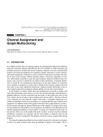
The network topology can be either one-dimensional or two-dimensional. As demonstrat-

ed in Figure 2.2, in one-dimensional topology, each cell has two neighboring cells if they
exist [17]. Some researchers use a ring topology in which the first and the last cells are
considered as neighboring cells [11]. The one-dimensional topology is used to model the
service area in which the mobility of mobile stations is restricted to either forward or
backward direction. Examples include highways and railroads.
The two-dimensional network topology is used to model a more general service area in
which mobile stations can move in any direction. There are two possible cell configura-
tions to cover the service area—hexagonal configuration and mesh configuration. The
hexagonal cell configuration is shown in Figure 2.1, where each cell has six neighboring
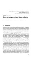
cells. Figure 2.3 illustrates a mesh cell configuration. Although eight neighbors can be as-
sumed for each cell in the mesh configuration, most researchers assume four neighbors
(horizontal and vertical ones only) [2, 3, 5, 22]. Although the mesh configuration has been
assumed for simplicity, it is not known whether the mesh configuration, especially the one
with four neighbors, is a practical model.
2.4.2 Call Arrival Probability
The call arrival probability plays a very important role when evaluating the performance
of a location management scheme. If the call arrival time is known to the called mobile
station in advance, the mobile station can update its location just before the call arrival
time. In this way, costs of both locate update and paging are kept to the minimum. Howev-
er, the reality is not like this. Many researchers assume that the incoming call arrivals to a
mobile station follow a Poisson process. Therefore, the interarrival times have indepen-
30
LOCATION MANAGEMENT IN CELLULAR NETWORKS
Figure 2.2 One-dimensional network topology.
dent exponential distributions with the density function f(t) =
␭
e
–
␭
t

[2, 19, 22]. Here
␭
rep-
resents the call arrival rate. Some researchers assume the discrete case. Therefore, the call
interarrival times have geometric distributions with the probability distribution function
F(t) = 1 – (1 –
␭
)
t
[1, 17, 24]. Here
␭
is the call arrival probability.
2.4.3 Mobility Models
The mobility pattern also plays an important role when evaluating the performance of a
location management scheme. A mobility model is usually used to describe the mobility
of an individual subscriber. Sometimes it is used to describe the aggregate pattern of all
subscribers. The following are several commonly used mobility models.
Fluid Flow Model
The fluid flow model has been used in [43] to model the mobility of vehicular mobile sta-
tions. It requires a continuous movement with infrequent speed and direction changes. The
fluid flow model is suitable for vehicle traffic on highways, but not suitable for pedestrian
movements with stop-and-go interruption.
Random Walk Model
Many researchers have used the discrete random walk as the mobility model. In this mod-
el, it is assumed that time is slotted, and a subscriber can make at most one move during a
time slot. Assume that a subscriber is in cell i at the beginning of time slot t. For the one-
dimensional network topology, at the beginning of time slot t + 1, the probability that the
subscriber remains in cell i is p, and the probability that the subscriber moves to cell i + 1
or cell i – 1 is equally (1 – p)/2 [11, 24].
The discrete random walk model has also been used in the two-dimensional network

topology [2, 17]. For the hexagonal configuration, the probability that the subscriber re-
mains in the same cell is p, and the probability that the subscriber moves to each neigh-
2.4 COMMON ASSUMPTIONS FOR PERFORMANCE EVALUATION
31
Figure 2.3 Two-dimensional network topology with the mesh configuration.
boring cell is equally (1 – p)/6. The concept of ring has been introduced to convert the
two-dimensional random walk to the one-dimensional one. A simplified two-dimensional
random walk model has been proposed in [5].
Markov Walk Model
Although the random walk model is memoryless, the current move is dependent on the
previous move in the Markov walk model. In [11], the Markov walk has been used to
model mobility in the one-dimensional ring topology. Three states have been assumed for
a subscriber at the beginning of time slot t: the stationary state (S), the left-move state (L),
and the right-move state (R). For the S state, the probability that the subscriber remains in
S is p, and the probability that the subscriber moves to either L or R is equally (1 – p)/2.
For the L (or R) state, the probability that the subscriber remains in the same state is q, the
probability that the subscriber moves to the opposite state is v, and the probability that the
subscriber moves to S is 1 – q – v. Figure 2.4 illustrates the state transitions.
In [12], the authors split the S state into SL and SR—a total of four states. Both SL and
SR are stationary, but they memorize the most recent move, either leftward (for SL) or
rightward (for SR). The probability of resuming motion in the same direction has been dis-
tinguished from that in the opposite direction.
Cell-Residence-Time-Based Model
While one group of researchers uses the probability that a mobile station may remain in
the same cell after each time slot to determine the cell residence time implicitly, another
group considers the cell residence time as a random variable [2, 19, 22]. Most studies use
the exponential distribution to model the cell residence time because of its simplicity. The
Gamma distribution is selected by some researchers for the following reasons. First, some
important distributions such as the exponential, Erlang, and Chi-square distributions are
special cases of the Gamma distribution. Second, the Gamma distribution has a simple

Laplace–Stieltjes transform.
32
LOCATION MANAGEMENT IN CELLULAR NETWORKS
Figure 2.4 The state transitions of the Markov walk model.
Gauss–Markov Model
In [21], the authors have used the Gauss–Markov mobility model, which captures the ve-
locity correlation of a mobile station in time. Specifically the velocity at the time slot n,
v
n
, is represented as follows:
v
n
=
␣
v
n–1
+ (1 –
␣
)
␮
+ ͙1
ෆ
–
ෆ
␣
ෆ
2
ෆ
x
n–1

Here 0 Յ
␣
Յ 1,
␮
is the asymptotic mean of v
n
when n approaches infinity, and x
n
is an
independent, uncorrelated, and stationary Gaussian process with zero mean. The
Gauss–Markov model represents a wide range of mobility patterns, including the constant
velocity fluid flow models (when
␣
= 1) and the random walk model (when
␣
= 0 and
␮
=
0).
Normal Walk Model
In [41], the authors have proposed a multiscale, straight-oriented mobility model referred
to as normal walk. They assume that a mobile station moves in unit steps on a Euclidean
plane. The ith move, Y
i
, is obtained by rotating the (i – 1)th move, Y
i–1
, counterclockwise
for
␪
i

degrees:
Y
i
= R(
␪
i
)Y
i–1
Here
␪
i
is normally distributed with zero mean. Since the normal distribution with zero
mean is chosen, the probability density increases as the rotation angle approaches zero.
Therefore, a mobile station has a very high probability of preserving the previous direc-
tion.
Shortest Path Model
In [3], the authors have introduced the shortest path model for the mobility of a vehicular
mobile station. The network topology used to illustrate the model is of the mesh configu-
ration. They assume that, within the location area, a mobile station will follow the shortest
path measured in the number of cells traversed, from source to destination. At each inter-
section, the mobile station makes a decision to proceed to any of the neighboring cells
such that the shortest distance assumption is maintained. That means that a mobile station
can only go straight or make a left or right turn at an intersection. Furthermore, a mobile
station cannot make two consecutive left turns or right turns.
Activity-Based Model
Instead of using a set of random variables to model the mobility pattern, an actual activity-
based mobility model has been developed at the University of Waterloo [38, 39]. The
model is based on the trip survey conducted by the Regional Municipality of Waterloo in
1987. It is assumed that a trip is undertaken for taking part in an activity such as shopping
at the destination. Once the location for the next activity is selected, the route from the

current location to the activity location will be determined in terms of cells crossed. The
2.4 COMMON ASSUMPTIONS FOR PERFORMANCE EVALUATION
33
activity-based mobility model has been used to test the performance of several popular lo-
cation management schemes [39]. It has shown that the scheme that performs well in a
random mobility model may not perform as well when deployed in actual systems.
2.5 LOCATION MANAGEMENT SCHEMES
2.5.1 Location Areas
The location areas approach has been used for location management in some first-genera-
tion cellular systems and in many second-generation cellular systems such as GSM [30].
In the location areas approach, the service coverage area is partitioned into location areas,
each consisting of several contiguous cells. The base station of each cell broadcasts the
identification (ID) of location area to which the cell belongs. Therefore, a mobile station
knows which location area it is in. Figure 2.5 illustrates a service area with three location
areas.
A mobile station will update its location (i.e., location area) whenever it moves into a
cell that belongs to a new location area. For example, when a mobile station moves from
cell B to cell D in Figure 2.5, it will report its new location area because cell B and cell D
are in different location areas. When an incoming call arrives for a mobile station, the cel-
lular system will page all cells of the location area that was last reported by the mobile sta-
tion.
The location areas approach is global in the sense that all mobile stations transmit their
location updates in the same set of cells, and it is static in the sense that location areas are
fixed [11, 33]. Furthermore, a mobile station located close to a location area boundary
will perform more location updates because it moves back and forth between two location
areas more often. In principle, a service area should be partitioned in such a way that both
the location update cost and the paging cost are minimized. However, this is not possible
34
LOCATION MANAGEMENT IN CELLULAR NETWORKS
Figure 2.5 A service area with three location areas.

because there is trade-off between them. Let us consider two extreme cases. One is known
as “always-update,” in which each cell is a location area. Under always-update, a mobile
station needs to update its location whenever it enters a new cell. Obviously, the cost of lo-
cation update is very high, but there is no paging cost because the cellular system can just
route an incoming call to the last reported cell without paging. The other is known as
“never-update,” in which the whole service area is a location area. Therefore there is no
cost of location update. However, the paging cost is very high because the cellular system
needs to page every cell in the service area to find out the cell in which the mobile is cur-
rently located so an incoming call can be routed to the base station of that cell.
Various approaches for location area planning in a city environment, the worst-case en-
vironment, are discussed in [25]. The simplest approach is the use of heuristic algorithms
for approximating the optimal location area configuration. The approach collects a high
number of location area configurations and picks up the best one. Although the approach
does not guarantee the optimal location area configuration, the optimal solution can be
approximated when the number of experiments is high. A more complex approach is
based on area zones and highway topology. A city can have area zones such as the city
center, suburbs, etc. Moreover, population movements between area zones are usually
routed through main highways that connect the area zones. Naturally, the size of a location
area is determined by the density of mobile subscribers, and the shape is determined by
the highway topology. Location updates due to zig-zag movement can be avoided if loca-
tion areas with overlapping borders are defined. The most complex approach is to create
dynamic location area configurations based on the time-varying mobility and traffic con-
ditions. For example, when the network detects a high-mobility and low-traffic time zone,
it decides to reduce the number of location areas to reduce location updates. When the net-
work detects an ordinary mobility and high-traffic time zone, it decides to increase the
number of location areas to reduce paging. The above approaches are based on the mobil-
ity characteristics of the subscriber population.
The authors in [25] also discussed location area planning based on the mobility charac-
teristics of each individual mobile subscriber or a group of mobile subscribers. Another
per-user dynamic location area strategy has been proposed in [43]. Their strategy uses the

subscriber incoming call arrival rate and mobility to dynamically determine the size of a
subscriber’s location area, and their analytical results show their strategy is better than sta-
tic ones when call arrival rates are subscriber- or time-dependent.
In the classical location area strategy, the most recently visited location area ID is
stored in a mobile station. Whenever the mobile station receives a new location area ID, it
initiates a location update. In [19], the author has proposed a two location algorithm
(TLA). The two location algorithm allows a mobile station to store the IDs of two most re-
cently visited location areas. When a mobile station moves into a new location area, it
checks to see if the new location is in the memory. If the new location is not found, the
most recently visited location is kept and the other location is replaced by the new loca-
tion. In this case, a location update is required to notify the cellular system of the change
that has been made. If the new location is already in the memory, no location update is
performed. When an incoming call arrives for a mobile station, two location areas are
used to find the cell in which the mobile station is located. The order of the locations se-
lected to locate the mobile station affects the performance of the algorithm. The possible
2.5 LOCATION MANAGEMENT SCHEMES
35