Tài liệu Multisensor thiết bị đo đạc thiết kế 6o (P2) doc

25
2
INSTRUMENTATION AMPLIFIERS
AND PARAMETER ERRORS
2-0 INTRODUCTION
This chapter is concerned with the devices and circuits that comprise the electronic
amplifiers of linear systems utilized in instrumentation applications. This develop-
ment begins with the temperature limitations of semiconductor devices, and is then
extended to differential amplifiers and an analysis of their parameters for under-
standing operational amplifiers from the perspective of their internal stages. This
includes gain–bandwidth–phase stability relationships and interactions in multiple
amplifier systems. An understanding of the capabilities and limitations of opera-
tional amplifiers is essential to understanding instrumentation amplifiers.
An instrumentation amplifier usually is the first electronic device encountered in
a signal acquisition system, and in large part it is responsible for the ultimate data
accuracy attainable. Present instrumentation amplifiers are shown to possess suffi-
cient linearity, CMRR, low noise, and precision for total errors in the microvolt
range. Five categories of instrumentation amplifier applications are described, with
representative contemporary devices and parameters provided for each. These para-
meters are then utilized to compare amplifier circuits for implementations ranging
from low input voltage error to wide bandwidth applications.
2-1 DEVICE TEMPERATURE CHARACTERISTICS
The elemental semiconductor device in electronic circuits is the pn junction; among
its forms are diodes and bipolar and FET transistors. The availability of free carriers
that result in current flow in a semiconductor is a direct function of the applied ther-
mal energy. At room temperature, taken as 20°C (293°K above absolute zero), there
is abundant energy to liberate the valence electrons of a semiconductor. These carri-
ers are then free to drift under the influence of an applied potential. The magnitude
Multisensor Instrumentation 6
␴
Design. By Patrick H. Garrett

Copyright © 2002 by John Wiley & Sons, Inc.
ISBNs: 0-471-20506-0 (Print); 0-471-22155-4 (Electronic)
of this current flow is essentially a function of the thermal energy instead of the ap-
plied voltage and accounts for the temperature behavior exhibited by semiconduc-
tor devices (increasing current with increasing temperature).
The primary variation associated with reverse biased pn junctions is the change
in reverse saturation current I
s
with temperature. I
s
is determined by device geome-
try and doping with a variation of 7% per degree centigrade both in silicon and ger-
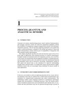
manium, doubling every 10°C rise. This behavior is shown by Figure 2-1 and equa-
tion (2-1). Forward-biased pn junctions exhibit a decreasing junction potential,
having an expected value of –2.0 mV per degree centigrade rise as defined by equa-
tion (2-2). The dV/dT temperature variation is shown to be the difference between
the forward junction potential V and the temperature dependence of I
s
. This rela-
tionship is the source of the voltage offset drift with temperature exhibited by semi-
conductor devices. The volt equivalent of temperature is an empirical model in both
equations defined as V
T
= (273°K + T °C)/11,600, having a typical value of 25 mV
at room temperature.
= I
s
· A/°C (2-1)
=
΂

– ·
΃
V/°C (2-2)
2-2 DIFFERENTIAL AMPLIFIERS
The first electronic circuit encountered by a sensor signal in a data acquisition sys-
tem typically is the differential input stage of an instrumentation amplifier. The bal-
anced bipolar differential amplifier of Figure 2-2(a) is an important circuit used in
many linear applications. Operation with symmetrical ± power supplies as shown
results in the input base terminals being at 0 V under quiescent conditions. Due to
the interaction that occurs in this emitter-coupled circuit, the algebraic difference
dI
s
ᎏ
dT
V
T
ᎏ
I
s
V
ᎏ
T
dV
ᎏ
dT
d(lnI
s
)
ᎏ
dT

dI
s
ᎏ
dT
26
INSTRUMENTATION AMPLIFIERS AND PARAMETER ERRORS
FIGURE 2-1. pn junction temperature dependence.
2-2 DIFFERENTIAL AMPLIFIERS
27
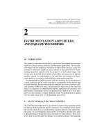
FIGURE 2-2. Differential DC amplifier and normalized transfer curves; h
fe
= 100, h
ie
= 1 k,
and h
oe
= 10
–6
.
⍀
signal applied across the input terminals is the effective drive signal, whereas equal-
ly applied input signals are cancelled by the symmetry of the circuit. With reference
to a single-ended output V
O
2
, amplifier Q
1
may be considered an emitter follower
with the constant current source an emitter load impedance in the megohm range.
This results in a noninverting voltage gain for Q

1
very close to unity (0.99999) that
is emitter-coupled to the common emitter amplifier Q
2
, where Q
2
provides the dif-
ferential voltage gain A
V
diff
by equation (2-3).
Differential amplifier volt–ampere transfer curves are defined by Figure 2-2(b),
where the abscissa represents normalized differential input voltage (V
1
– V
2
)/V
T
.
The transfer characteristics are shown to be linear about the operating point corre-
sponding to an input voltage swing of approximately 50 mV (± 1 V
T
unit). The
maximum slope of the curves occurs at the operating point of I
o
/2, and defines the
effective transconductance of the circuit as ⌬Ic/⌬(V
1
– V
2

)/V
T
. The value of this
slope is determined by the total current I
o
of equation (2-4). Differential input im-
pedances R
diff
and R
cm
are defined by equations (2-5) and (2-6). The effective volt-
age gain cancellation between the noninverting and inverting inputs is represented
by the common mode gain A
V
cm
of equation (2-7). The ratio of differential gain to
common mode gain also provides a dimensionless figure of merit for differential
amplifiers as the common mode rejection ratio (CMRR). This is expressed by equa-
tion (2-8), having a typical value of 10
5
.
A
V
diff
= single-ended V
O
2
(2-3)
= 50
I

o
= I
s
1
· exp(V
be
1
/V
T
) + I
s
2
· exp(V
be
2
/V
T
) (24)
= 1 mA
R
diff
= (2-5)
= 10 K
R
cm
= (2-6)
= 100 M
A
V
cm

= (2-7)
= 5 × 10
–4
h
oe
R
c
ᎏ
2
hfe
ᎏ
hoe
4V
T
h
fe
ᎏ
I
o
h
fe
R
c
ᎏ
2h
ie
28
INSTRUMENTATION AMPLIFIERS AND PARAMETER ERRORS
CMRR = (2-8)
= 10

5
The performance of operational and instrumentation amplifiers are largely de-
termined by the errors associated with their input stages. It is convention to ex-
press these errors as voltage and current offset values, including their variation
with temperature with respect to the input terminals, so that various amplifiers
may be compared on the same basis. In this manner, factors such as the choice of
gain and the amplification of the error values do not result in confusion con-
cerning their true magnitude. It is also notable that the symmetry provided by
the differential amplifier circuit primarily serves to offer excellent dc stability
and the minimization of input errors in comparison with those of nondifferential
circuits.
The base emitter voltages of a group of the same type of bipolar transistors at the
same collector current are typically only within 20 mV. Operation of a differential
pair with a constant current emitter sink as shown in Figure 2-2(a), however, pro-
vides a V
be
match of V
os
to about 1 mV. Equation (2-9) defines this input offset volt-
age and its dependence on the mismatch in reverse saturation current I
s
between the
differential pair. This mismatch is a consequence of variations in doping and geom-
etry of the devices during their manufacture. Offset adjustment is frequently provid-
ed by the introduction of an external trimpot R
V
os
in the emitter circuit. This permits
the incremental addition and subtraction of emitter voltage drops to 0 V
os

without
disturbing the emitter current I
o
.
Of greater concern is the offset voltage drift with temperature, dV
os
/dT. This in-
put error results from mistracking of V
be
1
and V
be
2
, described by equation (2-10),
and is difficult to compensate. However, the differential circuit reduces dV
os
/dT to 2
␮V/°C from the –2 mV/°C for a single device of equation (2-2), or an improvement
factor of 1/1000. By way of comparison, JFET differential circuit V
os
is on the order
of 10 mV, and dV
os
/dT typical1y 5 ␮V/°C. Minimization of these errors is achieved
by matching the device pinch-off voltage parameter. Bipolar input bias current off-
set and offset current drift are described by equations (2-11) and (2-12), and have
their genesis in a mismatch in current gain (h
fe
1
 h

fe
2
). JFET devices intrinsically
offer lower input bias currents and offset current errors in differential circuits,
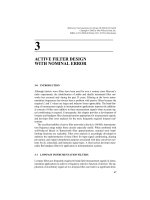
which is advantageous for the amplification of current-type sensor signals. Howev-
er, the rate of increase of JFET bias current with temperature is exponential, as il-
lustrated in Figure 2-3, and results in values that exceed bipolar input bias currents
at temperatures beyond 100°C, thereby limiting the utility of JFET differential am-
plifiers above this temperature.
V
os
= V
T
ln · (2-9)
= 1 mV
I
e
1
ᎏ
I
e
2
I
s
2
ᎏ
I
s
1
A

V
diff
ᎏ
A
V
cm
2-2 DIFFERENTIAL AMPLIFIERS
29
= – (2-10)
= 2 ␮V/°C
I
os
= I
b
1
– I
b
2
(2-11)
= 50 nA
= B · I
os
(2-12)
= 0.25 nA/°C
B = –0.005/°C > 25°C
= –0.015/°C < 25°C
dI
os
ᎏ
dT

dV
be
2
ᎏ
dT
dV
be
1
ᎏ
dT
dV
os
ᎏ
dT
30
INSTRUMENTATION AMPLIFIERS AND PARAMETER ERRORS
FIGURE 2-3. Device input bias current temperature drift.
2-3 OPERATIONAL AMPLIFIERS
Most operational amplifiers are of similar design, as described by Figure 2-4, and
consist of a differential input stage cascaded with a high-gain inner stage followed
by a power output stage. Operational amplifiers are characterized by very high
gain at dc and a uniform rolloff in this gain with frequency. This enables these de-
vices to accept feedback from arbitrary networks with high stability and simulta-
neous dc and ac amplification. Consequently, such networks can accurately impart
their characteristics to electronic systems with negligible degradation. The earliest
integrated circuit amplifier was offered in 1963 by Texas Instruments, but the
Fairchild 709 introduced in 1965 was the first operational amplifier to achieve
widespread application. Improvements in design resulted in second-generation de-
vices such as the National LM108. Advances in fabrication technology made pos-
sible amplifiers such as by the Analog Devices OP-07, with improved perfor-

mance overall. Subsequent refinements are represented by devices including the
Linear LTC-1250, featuring zero drift and ultralow noise. It is notable that con-
temporary operational amplifier circuits are structured around a high-gain inner-
stage employing a constant current source active load. The gain stage active load
impedance of approximately 500 K ohms ratioed with an emitter resistance R
e
approximating 100 ohms, shown in Figure 2-4, is responsible for high overall
A
V
o
.
2-3 OPERATIONAL AMPLIFIERS
31
FIGURE 2-4. Elemental operational amplifier.
Since
R
diff
Ǟ ϱ, V
d
= Ǟ 0 as |A
V
o
| Ǟ ϱ
A
V
c
= = = (2-13)
The circuit for an inverting operational amplifier is shown in Figure 2-5. The
cascaded innerstage gains of Figure 2-4 provide a total open-loop gain A
V

o
of
227,500, enabling realization of the ideal closed-loop gain A
V
c
representation of
equation (2-13). In practice, the A
V
o
value cannot be utilized without feedback be-
cause of nonlinearities and instability. The introduction of negative feedback be-
tween the output and inverting input also results in a virtual ground with equilibri-
um current conditions maintaining V
d
= V
1
– V
2
at zero. Classification of
operational amplifiers is primarily determined by the active devices that implement
the amplifier differential input. Table 2-1 delineates this classification.
According to negative feedback theory, an inverting amplifier will be unstable if
its gain is equal to or greater than unity when the phase shift reaches –l80° through
the amplifier. This is so because an output-to-input relationship will also have been
established, providing an additional –l80° by the feedback network. The relation-
ships between amplifier gain, bandwidth, and phase are described by Figure 2-6 and
–R
f
ᎏ
R

i
–IR
f
ᎏ
IR
i
V
o
ᎏ
V
s
V
o
ᎏ
A
V
o
32
INSTRUMENTATION AMPLIFIERS AND PARAMETER ERRORS
FIGURE 2-5. Inverting operational amplifier.
A
V
o
V
d