Tài liệu Đo lường quang học P10 ppt

10
Digital Image Processing
10.1 INTRODUCTION
The electronic camera/frame grabber/computer combination has made it easy to digitize,
store and manipulate images. These possibilities have made a great impact on optical
metrology in recent years. Digital image processing has evolved as a specific scientific
branch for many years. Many of the methods and techniques developed here are directly
applicable to problems in optical metrology. In this chapter we go through some of
the standard methods such as edge detection, contrast stretching, noise suppression, etc.
Besides, algorithms for solving problems specific for optical metrology are needed. Such
methods will be treated in Chapter 11.
10.2 THE FRAME GRABBER
A continuous analogue representation (the video signal) of an image cannot be conve-
niently interpreted by a computer and an alternative representation, the digital image,
must be used. It is generated by an analogue-to digital (A/D) converter, often referred
to as a ‘digitizer’, a ‘frame-store’ or a ‘frame-grabber’. With a frame grabber the digital
image can be stored into the frame memory giving the possibility of data processing and
display. The block diagram of a frame grabber module is shown in Figure 10.1. These
blocks can be divided into four main sections:
(1) the video source interface;
(2) multiplexer and input feedback LUT;
(3) frame memory;
(4) display interface.
The video source interface
The video source interface performs three main operations: (1) signal conditioning,
(2) synchronization/timing and (3) digitalization. In the signal condition circuitry the
signal is low-pass filtered with a cut-off frequency of 3–5 MHz to avoid aliasing, see
Section 5.8.3. Some frame grabbers also have programmable offset and gain.
Optical Metrology. Kjell J. G
˚
asvik

Copyright

2002 John Wiley & Sons, Ltd.
ISBN: 0-470-84300-4
250
DIGITAL IMAGE PROCESSING
Video
multiplexer
Data
multiplexer
Feedback
MUX
Input
feedback
LUT
Memory
frame
8-bit A/D
converter
Filter
Gain
Offset
D.C.
restore
12
12
12
12
12
12

12
8
Digital
input
Vision
bus
Video input
Synchronize
Camera
synchronize
Stripper
Crystal PLL
Pixel clock
System
timing
Synchronize
monitor
Synchronize
camera
Blue
Green
Red
DAC
8
8
8
12
12
12
12

LUT
Blue
LUT
Green
LUT
Red
Vision
bus
Figure 10.1 Block diagram of frame grabber
Before A/D conversion, the video signal must be stripped from its horizontal and
vertical sync signals. The pixel clock in the frame grabber defines the sampling interval
of the A/D converter and generates an internal Hsync signal. A phase-locked loop (PLL)
tries to match this Hsync with the Hsync signal from the camera by varying the pixel
clock frequency. This matching is iterative so it takes some time before the Hsyncs fit.
And even then this process keeps on oscillating and produce a phenomenon called line
jitter. Line jitter is therefore a mismatch and a wrong sampling of the analogue signal
and has its largest effect in the first TV lines (upper part of the picture). The error can
be as high as one pixel and therefore may ruin measurements which aims at subpixel
accuracy.
Most frame grabbers have an 8-bit flash converter but 12- and 16-bit converters exists.
The converter samples the analogue video signal at discrete time intervals and converts
each sample to a digital value called a pixel element or pixel. The incoming signal is an
analogue signal ranging from 0 to 714 mV at a frequency range from 7 to 20 MHz (with
no prefiltering). The 8-bit converter produces samples with intensity levels between 0 and
255, i.e. 256 different grey levels.
CAMERA CALIBRATION
251
Multiplexer and input feedback LUT
The frame memory of an 8-bit converter has a depth of 12 bits. The 4-bit spare allows the
processor to use look-up table (LUT) operations. The LUT transforms image data before

it is stored in the frame memory. The LUTs are mostly used for colouring (false colours)
of images and can also be used to draw graphics on the screen without changing the
underlying image. This can be done by protecting the lower 8 bits (the image) and draw
only in the upper 4 bits. It is therefore possible to grab a new image without destroying the
graphics. The LUT operations can be done in real time and its therefore possible to correct
images radiometrically before storing them. LUTs can not be used geometrically because
their memory is pixel organized, not space oriented. For geometrical transformations one
therefore has to make special programs. The multiplexer (MUX) in combination with the
feedback/input LUT allows some feedback operations like real-time image differencing,
low pass filtering, etc.
Frame memory
The frame memory is organized as a two-dimensional array of pixels. Depending on the
size of the memory it can store one or more frames of video information. When the
memory is a 12-bit memory, 8 bits are used for the image and 4 bit planes for generating
graphic overlay or LUT operations. In normal mode the memory acquires and displays
an image using read/modify/write cycles. The memory is XY addressed to have an easy
and fast access to single pixels.
Display interface
The frame memory transports the contents to the display interface every memory cycle.
The display interface transforms the digital 12-bit signal from the frame memory into an
analogue signal with colour information. This signal is passed to the RED, GREEN and
BLUE ports and from there to the monitor.
10.3 DIGITAL IMAGE REPRESENTATION
By means of an electronic camera and a frame grabber, an image will be represented
as a two-dimensional array of pixels, each pixel having a value g(x, y) between 0
and 255 representing the grey tone of the image in the pixel position. Most current
commercial frame grabbers have an array size of 512 × 512 pixels. Due to the way
the image is scanned, the customary XY coordinate axis convention is as indicated in
Figure 10.2.
10.4 CAMERA CALIBRATION

The calibration of the camera/lens combination is the process of determining the cor-
rect relationships between the object and image coordinates (Tsai 1987; Lenz and Tsai
1988). Since the elements of such a system are not ideal, this transformation includes
252
DIGITAL IMAGE PROCESSING
y
x
g (x, y)
(0,0)
Figure 10.2 Digital image representation
parameters that must be calibrated experimentally. Because we are mainly concerned with
relative measurements, we confine our discussion to three parameters that will affect our
type of measurements. That is lens distortion, image centre coordinates and perspective
transformations.
10.4.1 Lens Distortion
For an ideal lens, the transformation from object (x
o
,y
o
) to image (x
i
,y
i
) coordinates is
simply
x
i
= mx
o
(10.1a)

y
i
= my
o
(10.1b)
where m is the transversal magnification. It is well known, however, that real lenses
possesses distortion to a smaller or larger extent (Faig 1975; Shih et al. 1993). The
transfer from object to image coordinates for a distorting lens is (see Figure 10.3)
r
i
= mr
o
+ d
1
r
3
o
(10.2a)
where
r
i
=

x
2
i
+ y
2
i
,r

o
=

x
2
o
+ y
2
o
(10.2b)
Higher odd order terms of r
o
may be added, but normally they will be negligible. By
multiplying Equation (10.2a) by cos φ and sin φ,weget(sincex = r cos φ, y = r sin φ)
x
i
= mx
o
+ d
1
x
o
(x
2
o
+ y
2
o
) (10.3a)
y

i
= my
o
+ d
1
y
o
(x
2
o
+ y
2
o
) (10.3b)
This results in the well-known barrel (positive d
1
) and pin-cushion (negative d
1
) distortion.
CAMERA CALIBRATION
253
y
o
x
o
f
r
o
y
i

x
i
f
r
i
(a) (b)
Figure 10.3 (a) Object and (b) image coordinates
In a digital image-processing system we want to transform the distorted coordinates
(x
d
,y
d
) to undistorted coordinates (x
u
,y
u
). This transformation becomes
x
u
= x
d
+ dx
d
(x
2
d
+ ε
2
y
2

d
) (10.4a)
y
u
= y
d
+ dy
d
(x
2
d
+ ε
2
y
2
d
) (10.4b)
where ε is the aspect ratio between the horizontal and vertical dimensions of the pixels.
The origin of the xy-coordinates is at the optical axis. When transforming to the
frame-store coordinate system XY (see Section 10.3) by the transformation
x = X − X
s
(10.5a)
y = Y − Y
s
(10.5b)
Equation (10.4) becomes
X
u
= X

d
+ d(X
d
− X
s
)[(X
d
− X
s
)
2
+ ε
2
(Y
d
− Y
s
)
2
] (10.6a)
Y
u
= Y
d
+ d(Y
d
− Y
s
)[(X
d

− X
s
)
2
+ ε
2
(Y
d
− Y
s
)
2
] (10.6b)
where (X
s
,Y
s
) are the centre coordinates. The distortion factor d has to be calibrated by
e.g. recording a scene with known, fixed points or straight lines. The magnitude of d is
of the order of 10
−6
− 10
−8
pixels per mm
3
.
It has been common practice in the computer vision area to choose the center of
the image frame buffer as the image origin. For a 512 × 512 frame buffer that means
X
s

= Y
s
= 255. With a CCIR video format, the center coordinates would rather be (236,
255) since only the first 576 of the 625 lines are true video signals, see Table 5.4. A
mispositioning of the sensor chip in the camera could add further to these values. The
problem is then to find the coordinates of the image center. Many methods have been
proposed, one which uses the reflection of a laser beam from the frontside of the lens
(Tsai 1987). When correcting for camera lens distortion, correct image center coordinates
are quite important.
254
DIGITAL IMAGE PROCESSING
Image
plane
Object
plane
−
x
i
x
i
x
o
x
o
x
p
z
p
z
a

b
Figure 10.4 Perspective transformation
10.4.2 Perspective Transformations
Figure 10.4 shows a lens with the conjugate object- and image planes and with object and
image distances a and b respectively. A point with coordinates (x
p
,z
p
) will be imaged
(slightly out of focus) with image coordinate −x
i
, the same as for the object point (x
o
, 0).
From similar triangles we find that
x
p
=
−x
i
(z
p
+ a)
b
(10.7a)
y
p
=
−y
i

(z
p
+ a)
b
(10.7b)
Equation (10.7) is the perspective transformation and must be taken into account when
e.g. comparing a real object with an object generated in the computer.
10.5 IMAGE PROCESSING
Broadly speaking, digital image processing can be divided into three distinct classes of
operations: point operations, neighbourhood operations and geometric operations. A point
IMAGE PROCESSING
255
operation is an operation in which the grey level of each pixel in the output image is
a function of the grey level of the corresponding pixel in the input image, and only of
that pixel. Typical point operations are photometric decalibration, contrast stretching and
thresholding. A neighbourhood operation generates an output pixel on the basis of the grey
level of the corresponding pixel in the input image and its neighbouring pixels. Geometric
operations change the spatial relationships between points in an image, i.e. the relative
distances between points a, b and c will typically be different after a geometric operation or
‘warping’. Correcting lens distortion is an example of geometric operations. Digital image
processing is a wide and growing topic with an extensive literature (Vernon 1991; Baxes
1994; Niblack 1988; Gonzales and Woods 2002; Pratt 1991; Rosenfeld and Kak 1982).
Here we’ll treat only a small piece of this large subject and specifically consider operation,
which can be very useful for enhancing interferograms, suppress image noise, etc.
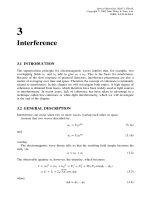
10.5.1 Contrast Stretching
In a digitized image we may take the number of pixels having the same grey level and
make a plot of this number of pixels as a function of grey level. Such a plot is called
a grey-level histogram. For an 8-bit (256 grey levels) image it may look such as that
in Figure 10.5(a). In this example the complete range of grey levels is not used and the
contrast of this image will be quite poor. We wish to enhance the contrast so that all

levels of the grey scale are utilized. If the highest and lowest grey value of the image are
denoted g
H
and g
L
respectively, this is achieved by the following operation:
20 40 60 80 100 120
Grey level
(a)
(b)
140 160 180 200 220 240 255
Number of pixels
20 40 60 80 100 120
Grey level
140 160 180 200 220 240 255
Number of pixels
Figure 10.5 Grey-level histogram (a) before and (b) after contrast stretching