Tài liệu Đo lường quang học P11 pptx

11
Fringe Analysis
11.1 INTRODUCTION
In Chapters 3 and 6–9 we have given a description of classical interferometry, holographic
interferometry, moir
´
e, speckle and photoelasticity. The outcome of all these techniques is
a set of fringes called interferograms. For many years, the analysis of these interferograms
has been a matter of manually locating the positions and numbering of the fringes. With
the development and decreasing cost of digital image processing equipment, a lot of effort
has been made into what is termed digital fringe pattern measurement techniques. It is
three main reasons for this effort: (1) to obtain better accuracy; (2) to increase the speed;
(3) to automate the process.
In this chapter, some of the basic principles of digital fringe pattern analysis will be
described. In Section 11.2 we describe techniques which intend to be a direct replace-
ment of the human brain – eye combination by detecting the positions of the fringes. In
Sections 11.3, 11.4 and 11.5, techniques for continuous determination of the phase of
the fringe function are described. For more detailed discussions of digital fringe pattern
measurement techniques, the book edited by Robinson and Reid (1993) is recommended.
A comparison of the different techniques is performed by Kujawinska 1993b and Perry
and McKelvie (1993).
11.2 INTENSITY-BASED ANALYSIS METHODS
11.2.1 Introduction
Before the development of the phase-measurement techniques described in Sections 11.3
and 11.4, intensity-based techniques were the only image-processing tools available for the
automatic analysis of interferograms. They still are important methods in fringe analysis
and are sometimes the only viable technique for interferograms which have been retrieved
from photographic records or which have been obtained from interferometers in which it
is impossible or impractical to introduce phase-measuring techniques. They may also be
appropriate simply because quantitative results are not even needed.
For intensity-based methods it is very important to minimize the influence of noise,

including speckle noise. Therefore preprocessing of the interferograms is highly recom-
mended. Techniques most commonly used and described in Section 10.5.3 are low-pass
filtering and median filtering. Specially designed for fringe analysis are the so-called
Optical Metrology. Kjell J. G
˚
asvik
Copyright

2002 John Wiley & Sons, Ltd.
ISBN: 0-470-84300-4
270
FRINGE ANALYSIS
spin-filters (Yu et al. 1994). Another method (if possible) is to combine two interferograms
of opposite phase. When an interferogram is shifted in phase by π radians, the resulting
dark fringes occupy the previous location of bright fringes and vice versa. If the noise
is stationary, the noise distribution is unaffected by this shift. Then if the two interfero-
grams are subtracted, the noise will subtract to give zero, while the fringes will combine
to give a higher contrast than in the original. When the noise has approximately the
same spatial frequency as the fringes, this method might be the only workable one for
noise reduction.
11.2.2 Prior Knowledge
When interferometric techniques are used for repetitive calibration, non-destructive testing
or inspection, it is sometimes possible to design a comparatively simple fringe analysis
system. After identifying the characteristics of the fringe pattern which are peculiar to the
application, the capabilities of the analysis system can then be confined to those required
for the measurement in question.
A very simple analysis method can be applied to moir
´
e technique using projected
fringes where the shape of a manufactured component can be compared with that of a

master component. For a manufactured component identical to the master, the resulting
image becomes uniformly dark. As the manufactured component deviates from the master,
fringes appear in the image and hence the total intensity of the image increases. Der
Hovanesian and Hung (1982) used this technique to control component shape by limiting
the total image intensity to a threshold value.
Many specialised fringe analysis procedures can be developed by utilizing prior knowl-
edge of the fringe pattern. The Young fringe method (see Section 8.4.2) resulting in a
set of parallel fringes is a typical example which has undergone a lot of investigations
(Halliwell and Pickering (1993)). Another example is holographic interferometry applied
to testing of honeycomb panels (Robinson 1983). Debrazing of the honeycomb produces
groups of nearly circular fringes of a particular size and fringe density. As shown in
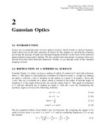
Figure 11.1 the procedure starts with counting the number of fringes along a number of
horizontal lines through the image. When a comparatively large number of fringes appear
on a given line, a flaw is presumed to exist on that line. Short vertical scans along the
line are then used to search for the location of the flaw by looking for a comparatively
large number of fringes in the vertical direction. Having identified the probable exis-
tence and location of a flaw, the system carries out a further check by counting fringes
along each of four short vectors angularly spaced at 45
◦
, centred on the probable flaw
site. If the same number of fringes appear on each of the four vectors, then the exis-
tence of a flaw is confirmed. As shown in Figure 11.2 the flaw sites are marked with
small crosses.
11.2.3 Fringe Tracking and Thinning
Boundary (contour) tracking and object thinning (skeletoning) are standard operations
in digital image processing. In fringe analysis we talk about fringe tracking and thin-
ning, which have a slightly different meaning. A number of fringe tracking and thinning
procedures have been proposed.
INTENSITY-BASED ANALYSIS METHODS
271

N = 512
∆N
<>
Count fringe peaks
along horizontal
vectors
Count peaks along
vertical vectors
(a)
(b)
(c)
Scan at 0°, 90°, 45°
and 135°
Figure 11.1 Procedure for the analysis of Figure 11.2 (From Robinson, D. W. (1983) Automatic
fringe analysis with a computer image processing system, Applied Optics, 22, 2169–76. Reproduced
by permission of The Optical Society of America and by Courtesy of D. W. Robinson)
Figure 11.2 Result of analysing a holographic interferogram by the method shown in Figure 11.1
(From Robinson, D. W. (1983) Automatic fringe analysis with a computer image processing system,
Applied Optics, 22, 2169–76. Reproduced by permission of the Optical Society of America and
by Courtesy of D. W. Robinson)
272
FRINGE ANALYSIS
Fringe tracking involves a search for the locus of the fringe maxima (or minima)
by examining the pixel values in all directions from the starting point (often deter-
mined manually) and moving the pixel locus in the direction along which the sum of
the intensity is maximized (or minimized) or alternatively the gradient is a minimum. (As
opposed to boundary tracking where one searches for the maximum gradient value.) In
this way only a limited set of the whole image array is examined (Button et al. 1985),
see Figure 11.3.
Thinning and skeletonizing techniques use similar approaches to detect fringe peaks

(or minima) but instead of following the peaks with a roving pixel locus, the whole image
is subjected to a peak detection matrix. A procedure due to Yatagai et al. (1982) uses
two-dimensional peak detection, locally performed within a 5 × 5 pixel matrix as shown
in Figure 11.4(a). With respect to the four directions shown in Figure 11.4(b), the peak
conditions are defined as
P
00
+ P
0−1
+ P
01
>P
−21
+ P
−20
+ P
−2−1
P
00
+ P
0−1
+ P
01
>P
21
+ P
20
+ P
2−1
(11.1)

for the x-direction, with similar expressions for the y-direction and the xy-andyx-direc-
tions. When the peak conditions are satisfied for any two or more directions, the object
point is recognized to be a point on a fringe skeleton.
Figure 11.3 Holographic interferogram with a computer tracked fringe. (From Button, B. L.,
Cutts, J., Dobbins, B. N., Moxan, G. J. and Wykes, C. (1985) The identification of fringe posi-
tions in speckle patterns, Opt. and Lasers Technology, 17, 189– 92. Reproduced by permission of
Elsevier Science Ltd)
INTENSITY-BASED ANALYSIS METHODS
273
P
−22
P
−12
P
02
P
12
P
22
−
xy
xy
x
y
(a) (b)
P
−21
P
−11
P

01
P
11
P
21
P
−20
P
−10
P
00
P
10
P
20
P
−2−1
P
−1−1
P
0−1
P
1−1
P
2−1
P
−2−2
P
−1−2
P

0−2
P
1−2
P
2−2
Figure 11.4 (a) 5 × 5 pixel matrix and (b) directions for fringe peak detection
11.2.4 Fringe Location by Sub-Pixel Accuracy
By the methods described above, fringes are located with an accuracy of one pixel. We
now describe two methods by which fringe positions can be determined with an accuracy
of a fraction of a pixel. The first method consists off fitting a curve around the fringe
maximum (or minimum)
Curve fitting
Assume that the intensity distribution of the fringe pattern locally is given by
I(x)= a + b cos
2π
p
(x − x
0
)(11.2)
with a maximum at x = x
0
,i.e.x
0
= np where n is an integer. Near the maximum we
can approximate the intensity by a Taylor expansion of the intensity around x
0
up to the
second order:
I(x)= a + b


1 −
1
2

2π
p

2
x
2

(11.3)
In Appendix D it is shown how such a quadratic curve can be fitted to N observation
points by using the least squares solution. By using three observation points I(i− 1),
I(i) and I(i+ 1) where i is the pixel number with the highest intensity I(i), the position
of the fringe maximum is given by, cf. Equation (D.19):
x
max
= i +
I(i− 1) − I(i+ 1)
2I(i− 1) − 4I(i)+ 2I(i+ 1)
(11.4)
Thereby determining the position with sub-pixel accuracy.
The accuracy of this method is, among other things, dependent on the fringe period p.
By using three measuring points, the length of p should at least be six pixels. If p is
274
FRINGE ANALYSIS
much longer than six pixels, it will be a good idea to fit the curve to four or more
measurement points. It could also be advantageous to include four and higher-order terms
in the expression for the intensity.

Zero-crossing
Another method for sub-pixel location of fringe maxima (or minima) is to find the points
where the intensity crosses the mean intensity value (G
˚
asvik et al. 1989). The principle is
shown in Figure 11.5. On the left side of the maximum, the last pixel x
lu
with intensity
I(x
lu
) below the mean intensity I
m
and the first pixel x
lo
with intensity I(x
lo
) over I
m
is
found. Then a straight line
I =
I(x
lo
) − I(x
lu
)
x
lo
− x
lu

x +
I(x
lu
)x
lo
− I(x
lo
)x
lu
x
lo
− x
lu
= [I(x
lo
) − I(x
lu
)]x + [I(x
lu
) − I(x
lo
)]x
lu
+ I(x
lu
) (11.5)
connecting the two points is calculated. (The last equality follows since x
lo
− x
lu

= 1.)
The intersection between this line and the mean intensity I
m
is given by
x
l
=
I
m
− I(x
lu
)
I(x
lo
) − I(x
lu
)
+ x
lu
(11.6)
I
(
x
lo
)
I
(
x
ro
)

I
(
x
ru
)
I
(
x
lu
)
x
lu
x
lo
x
ro
x
ru
x
l
x
m
x
r
I
m
Figure 11.5 Illustration of the detection of the crossover points x
l
and x
r

with the mean intensity I
m
INTENSITY-BASED ANALYSIS METHODS
275
In the same way, the crossover point x
r
on the right side of the maximum is found to be
x
r
=
I
m
− I(x
ru
)
I(x
ru
) − I(x
ro
)
+ x
ru
(11.7)
where x
ro
is the last pixel with intensity I(x
ro
) over I
m
and x

ru
is the first pixel with
intensity I(x
ru
) below I
m
. The position x
m
of the fringe maximum is then taken to be the
midpoint
x
m
=
x
l
+ x
r
2
=
1
2

I
m
− I(x
lu
)
I(x
lo
) − I(x

lu
)
−
I
m
− I(x
ru
)
I(x
ro
) − I(x
ru
)

+
x
lu
+ x
ru
2
(11.8)
The mean intensity can be found in different ways. From Figure 11.6 we see that the area
under the intensity curve and the area under the straight line
I
m
= ax + b(11.9)
representing the mean intensity should be approximately equal. If the interval from x
1
to
x

3
is divided into two equal subintervals at x
2
,wehave
a =
4(A
2
− A
1
)
N
2
(11.10a)
b =
3A
1
− A
2
N
−
4(A
2
− A
1
)
N
2
x
1
(11.10b)

where N = x
3
− x
1
, A
1
is the area of the first interval from x
1
to x
2
and A
2
is the area
of the second interval from x
2
to x
3
. These areas are found by simply taking the sum of
the intensities for each pixel
A
1
=
x
2

i=x
1
I
i
(11.11a)

A
2
=
x
3

i=x
2
I
i
(11.11b)
I
I
m

=
ax
+
b
x
1
x
2
A
1
A
2
x
3
x

Figure 11.6 Intensity distribution and mean intensity I
m
along a TV line
276
FRINGE ANALYSIS
To get the best possible representation of the mean intensity, each scan should be divided
into as many intervals as possible, giving a sequence of straight lines representing I
m
.
Each subinterval must however not be shorter than one fringe period.
Another way of calculating the mean intensity is by the so-called bucket and bin
method (Choudry 1981). It consists of finding the value of I
min
and I
max
(to the nearest
integer pixel) for successive minima and maxima and then taking I
m
= (I
max
+ I
min
)/2.
For fringes with a high level of noise it could however be difficult to discriminate against
spurious maxima and minima.
The accuracy of the zero-crossing method has been analysed with respect to the error
in I
m
and the fringe period (G
˚

asvik and Robbersmyr 1994). It shows that the absolute
accuracy is highest for a fringe period of six pixels, while the relative accuracy is relatively
constant for fringe periods of six pixels and higher. This analysis is done assuming noise-
free fringes.
For more details about intensity-based analysis methods, see Yatagai (1993).
11.3 PHASE-MEASUREMENT INTERFEROMETRY
11.3.1 Introduction
By means of a digital image-processing system, we have the possibility of storing an image
of the interferogram into the computer memory and do manipulations on the individual
pixels. When looking at the general expression for an interferogram, Equation (3.7):
I = I
1
+ I
2
+ 2

I
1
I
2
|γ| cos φ (11.12)
it would be tempting to solve this expression with respect to φ and let the com-
puter calculate:
φ = cos
−1
I − (I
1
+ I
2
)

2
√
I
1
I
2
|γ|
(11.13)
thereby calculating the phase at each pixel, and by knowledge of the geometrical and
optical configuration of the interferometer, calculating the parameter sought in each pixel
of the whole image. To do this, we see from Equation (11.13) that we must know the
intensities I
1
and I
2
and the degree of mutual coherence |γ| of the interfering waves,
and, moreover, we must know these quantities for each pixel. This assumption is unre-
alistic in most cases, and even if we knew these quantities of the ideal interferogram,
the intensity distribution from a complex imaging system will always be accompanied by
uncontrollable noise. In this section and in Sections 11.4 and 11.5 we will treat methods
that are dependent only on the recorded intensity at each pixel and which are less sensitive
to noise.
11.3.2 Principles of TPMI
A general expression for the recorded intensity in an interferogram can be written:
I(x, y) = a(x,y)+ b(x, y)cos φ(x,y) (11.14)
PHASE-MEASUREMENT INTERFEROMETRY
277
where both I , a, b and φ are functions of the spatial coordinates. Here a(x,y) is the
mean intensity, V = a(x,y)/b(x, y) is equal to the visibility (see Section 3.4) and φ is
the phase difference between the interfering waves.

To recover the phase we now describe a group of methods called phase-measurement
interferometry (PMI). PMI is the most widely used technique today for the measurement of
wavefront phase in interferometers and it has also been successfully applied in holographic
interferometry and moir
´
e (Rosvold 1990; Takeda and Mutoh 1983). PMI techniques can
be divided into two main categories: those which take the phase data sequentially, and
those which take the phase data simultaneously. Methods of the first type are known as
temporal PMI or TPMI, and those of the second type are known as spatial PMI and will
be treated in Section 11.4.
The starting point for all PMI techniques is the expression for the interferogram
intensity:
I = a + b cos(φ + α) (11.15)
where we have introduced an additional phase term α. The essential feature of all
PMI techniques is that α is a modulating phase which is introduced and controlled
experimentally.
Techniques for determining the phase can be split into two basic categories: electronic
and analytic. For analytical techniques, intensity data are recorded while the phase is
temporally modulated, sent to a computer and then used to compute the relative inten-
sity measurements. Electronic techniques are also known as heterodyne interferometry,
see Section 3.6.4. An example of this technique is described in Section 3.6.3 about the
dual-frequency Michelson interferometer. This method is used extensively in distance-
measuring interferometers where the phase at a single point with a fast update is required.
But the technique can also be used to determine the phase over an area, see Section 6.8.3.
The detector then has to be scanned or there must be multiple detectors with all the
necessary circuitry.
The analytic methods can be subdivided into two techniques, one that integrates the
intensity while the phase is increased linearly, and a second where the phase is altered
in steps between intensity measurements. The first method is referred to as integrating
bucket phase-shifting, while the second is termed phase-stepping. The phase-step method

has clearly become the most popular in recent years and below we give a brief description
of this technique.
Equation (11.15) contains three unknowns, a, b and φ, requiring a minimum of three
intensity measurements to determine the phase. The phase shift between adjacent mea-
surements can be anything between 0 and π degrees. By arbitrary phase shifts α
1
, α
2
and
α
3
we get
I
1
= a + b cos(φ + α
1
)
I
2
= a + b cos(φ + α
2
) (11.16)
I
3
= a + b cos(φ + α
3
)
from which we find
φ = tan
−1

(I
2
− I
3
) cos α
1
− (I
1
− I
3
) cos α
2
+ (I
1
− I
2
) cos α
3
(I
2
− I
3
) sin α
1
− (I
1
− I
3
) sin α
2

+ (I
1
− I
2
) sin α
3
(11.17)
278
FRINGE ANALYSIS
With α
1
= π/4, α
2
= 3π/4, α
3
= 5π/4, i.e. a phase shift of π/2 per exposure, we reach
a particularly simple expression
φ = tan
−1
I
2
− I
3
I
2
− I
1
(11.18)
Three intensity measurements to solve for φ gives an exactly determined system. As
mentioned in Appendix D, this often gives numerically unstable solutions and it is often

wise to overdetermine the system by providing more measurement points.
In general, for the ith stepped phase, the resulting intensity can be written as
(Greivenkamp 1984; Morgan 1982)
I
i
= a + b cos(φ + α
i
) = a
0
+ a
1
cos α
i
+ a
2
sin α
i
(11.19a)
where
a
0
= a = I
0
a
1
= b cos φ (11.19b)
a
2
=−b sin φ
By making N phase steps (i = 1, 2,...,N), Equation (11.19a) can be written in matrix

form as





I
1
I
2
.
.
.
I
N





=





1cosα
1
sin α
1

1cosα
2
sin α
2
.
.
.
.
.
.
.
.
.
1cosα
N
sin α
N







a
0
a
1
a
2



(11.20)
The coefficients a
0
, a
1
and a
2
can be found using the least squares solution to
Equation (11.20), see Appendix D


a
0
a
1
a
2


= A
−1
B(11.21)
where
A =


Ncos α
i

 sin α
i
 cos α
i
 cos
2
α
i
 cos α
i
sin α
i
 sin α
i
 cos α
i
sin α
i
 sin
2
α
i


(11.22)
and
B =


I

i
I
i
cos α
i
I
i
sin α
i


(11.23)
PHASE-MEASUREMENT INTERFEROMETRY
279
From Equation (11.19b) we find that
φ = tan
−1

−a
2
a
1

(11.24)
V =
b
a
=

a

2
1
+ a
2
2
a
0
(11.25)
We include the expression for the visibility because pixels with too low visibility can give
invalid phase data.
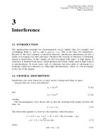
11.3.3 Means of Phase Modulation
A phase shift or modulation in an interferometer can be induced by moving a mirror, tilting
a glass plate, moving a grating, rotating a half-wave plate or analyzer (see Figure 11.7)
using an acousto-optic or electro-optic modulator, or using a Zeeman laser. Phase shifters
such as moving mirrors, gratings, tilted glass plates, or polarization components (Jin
et al. 1994) can produce continuous as well as discrete phase shifts between the object
and reference beams. Phase shifters may either be placed in one arm of the interferometer
or positioned so that they shift the phase of one of two orthogonally polarized beams.
11.3.4 Different Techniques
From Equations (11.20)–(11.25) we can derive the expressions for different
techniques, e.g.
PZT
(a)
First order
Polarized light
(b)
(c) (d)
Figure 11.7 Means of modulating or shifting the phase of the light in an interferometer (a) moving
mirror, (b) tilted glass plate; (c) moving diffraction grating; (d) rotating waveplate