Tài liệu Nguyên tắc phân tích tín hiệu ngẫu nhiên và thiết kế tiếng ồn thấp P8 pptx
Bạn đang xem bản rút gọn của tài liệu. Xem và tải ngay bản đầy đủ của tài liệu tại đây (309.67 KB, 27 trang )
8
Linear System Theory
8.1 INTRODUCTION
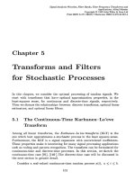
In this chapter, the fundamental relationships between the input and output of
a linear time invariant system, as illustrated in Figure 8.1, are detailed.
Specifically, the relationships between the input and output time signals,
Fourier transforms and power spectral densities, are established. Such relation-
ships are fundamental to many aspects of system theory, including analysis of
noise in linear systems, and low noise amplifier design.
The relationships between the parameters defined in Figure 8.1, and proved
in this chapter are,
y(t) :
R
x()h(t 9 ) d (8.1)
Y (T, f ) H(T, f )X(T, f ) (8.2)
where X and Y are the respective Fourier transforms, evaluated on the interval
[0, T ], of the signals x and y. However, as will be shown in this chapter, the
relationship defined in Eq. (8.2) is an approximation. If both x, h + L , then the
relative error in this approximation can be made arbitrarily small by making
T sufficiently large. However, stationary random signals are not Lebesgue
integrable on the interval (0, -) and hence, this convergence is not guaranteed.
However, it is shown, for a broad class of signals and random processes,
including periodic signals and stationary random processes, that the corre-
sponding relationship between the input and output power spectral densities,
namely,
G
7
(T, f ) "H(T, f )"G
6
(T, f ) (8.3)
becomes exact as T increases without bound. Establishing the relationships, as
per Eqs. (8.1)—(8.3), for a linear time invariant system requires the system
impulse response to be defined, and this is the subject of the next section.
229
Principles of Random Signal Analysis and Low Noise Design:
The Power Spectral Density and Its Applications.
Roy M. Howard
Copyright
2002 John Wiley & Sons, Inc.
ISBN: 0-471-22617-3
x ∈ E
X
G
X
G
Y
h ↔ H
y ∈ E
Y
Figure 8.1 Schematic diagram of a linear system. E
X
and E
Y
, respectively, represent the
ensemble of input and output signals. H is the Fourier transform of the impulse response
function h. G
X
and G
Y
, respectively, are the power spectral densities of the input and output
random processes.
∆
t
∞
∫
–∞
δ
∆
(t)dt = 1
δ
∆
(t)
1
∆
−
Figure 8.2 Definition of the function
.
8.2 IMPULSE RESPONSE
Fundamental to defining the impulse function of a time invariant linear system,
is the function
defined by the graph shown in Figure 8.2. The response of a
linear time invariant system to the input signal
is denoted h
.
D:I R By definition, the impulse response of a linear
system is the output signal, in response to the input signal
,as becomes
increasingly small, that is,
h(t) : lim
h
(t) (8.4)
8.2.1 Restrictions on Impulse Response
General requirements on the impulse function are, first, that it is integrable,
that is, h + L [0, -], and second, that as ; 0, the integrated difference between
h and h
is negligible on sets of nonzero measure, that is, convergence in the
mean over (0, -):
lim
"h
(t) 9 h(t)"dt : 0 (8.5)
230
LINEAR SYSTEM THEORY
t
i
i
β
i − 1
i + 1
i +
i
1 + 3β ⁄ 2
1
Figure 8.3 Illustration of a function that is Lebesgue integrable on [0, -], but is not square
Lebesgue integrable on the same interval.
The following are two examples where, as ; 0, the integrated error between
h and h
is finite. First, the ‘‘identity’’ system where h
(t) :
(t) and second,
the system where
h
(t) :
0
t+ [, ; 1/]
elsewhere
(8.6)
For both systems, and for t + (0, -), it follows that
h(t) : lim
h
(t) : 0 but lim
"h
(t) 9 h(t)"dt " 0 (8.7)
To ensure h + L [0, -], and as ; 0 the integrated difference between h and h
is negligible, the following restriction on the set of functions +h
,, denoted
condition 1, is sufficient:
1. There exists a function g + L [0, -], such that, for all 90 it is the case
that "h
(t)"-g(t) for t + [0, -].
The validity of this condition, in terms of guaranteeing that Eq. (8.5) holds, is
given by Theorem 2.25.
Practical and stable systems are such that h
is bounded and has finite
energy for all values of . As per Theorem 2.14 these two criteria are met by
condition 1 and the following condition.
2. For 90, h
is bounded, that is, 90, "h
(t)"-h
for t+ [0, -].
This second condition excludes a signal such as 1/(t
, which is integrable
on [0, -], but has infinite energy on all intervals of the form [0, t
M
]. It
also excludes signals such as the one shown in Figure 8.3, whose integral
equals
G
(1/i>@), which from the comparison test (Knopp, 1956
pp. 56f ), is finite for 90, but whose energy is given by
G
(1/i\@) and is
infinite when 90.
IMPULSE RESPONSE
231
8.3 INPUT ‒OUTPUT RELATIONSHIP
Consider the causal linear time invariant system illustrated in Figure 8.1. The
well-known relationship between the input and output signals is specified in
the following theorem.
T 8.1. I—O R L S If the
input signal x to, and the system impulse response h of, a linear time invariant
system are both causal, are locally integrable, and have bounded variation on all
finite intervals, then the output signal, y, is given by
y(t) :
R
x()h(t 9 ) d t 9 0 (8.8)
Proof. The proof of this result is given in Appendix 1.
Note that this result is applicable to unstable systems where h, L [0, -].
8.4 FOURIER AND LAPLACE TRANSFORM OF OUTPUT
The following theorem states the important result of the relationship between
the Fourier and Laplace transforms of the input and output of a linear time
invariant system.
T 8.2. T O S L S If both
x,h+ L [0, T ], have bounded variation on [0, T ], and their respective Fourier
transforms are denoted X and H, then the Fourier transform Y of the output
signal y, evaluated on [0, T ], is given by
Y (T, f ) :
WNH2
N>HW2
x()h(p)e\HLDN>H d dp
(8.9)
: Y
(T, f ) 9 I(T, f ) : X(T, f )H(T, f ) 9 I(T, f )
where
Y
(T, f ) : X(T, f )H(T, f )
(8.10)
I(T, f ) :
WNH2
N>H2
x()h(p)e\HLDN>H d dp
232
LINEAR SYSTEM THEORY
Figure 8.4 Illustration of area of integration for Y and I.
and the integration regions for both Y and I are as shown in Figure 8.4.
W ith
X(T, s) :
2
x(t)e\QR dt (8.11)
and similarly for other L aplace transformed variables, it is the case that
Y (T, s) :
WNH2
N>HW2
x()h(p)e\QN>H d dp
(8.12)
: X(T, s)H(T, s) 9 I(T, s)
where
I(T, s) :
WNH2
N>H2
x()h(p)e\QN>H d dp (8.13)
Proof. The proof of this theorem is given in Appendix 2.
For the Fourier transform case Y
(T, f ), because of its simplicity, is the
approximation that is normally used, and I(T, f ) is clearly the error between
the approximate and true output Fourier transforms for a given frequency f.
The next theorem gives a sufficient condition for the term I to approach zero
as the interval under consideration becomes increasingly large.
T 8.3 C A If both x, h + L [0, -], and
have bounded variation on all closed finite intervals, then
lim
2
Y (T, f ) : lim
2
X(T, f )H(T, f ) f + R (8.14)
lim
2
Y (T, s) : lim
2
X(T, s)H(T, s) Re[s] . 0 (8.15)
FOURIER AND LAPLACE TRANSFORM OF OUTPUT
233
t
T
t
T
t
T
x(t) h(t) y(t)
2T
Figure 8.5 Illustration of waveforms in a linear system for the case where the impulse
response and the input are windowed but the output is not.
Further, if h + L [0, -], x is locally integrable and does not exhibit exponential
increase, then Re[s] 9 0 is a sufficient condition for
lim
2
Y (T, s) : lim
2
X(T, s)H(T, s) (8.16)
Proof. The proof is given in Appendix 3.
8.4.1 Windowed Input and Nonwindowed Output
For completeness, the response of a linear time invariant system for the case
where the input and impulse response are windowed, but the output is not
windowed, as illustrated in Figure 8.5, is stated in the following theorem.
T 8.4 T O S:N C If both
x, h + L [0, T ], and have bounded variation on [0, T ], then the Fourier and
L aplace transforms Y
of the output signal y, which is not windowed, are given by
Y
(2T, f ) : X(T, f )H(T, f ) (8.17)
Y
(2T, s) : X(T, s)H(T, s)(8.18)
Proof. The proof of this result is given in Appendix 4.
This result has application, when the output signal y is to be derived for the
interval [0, T ]. The procedure is as follows for the Fourier transform case.
First, evaluate X(T, f ) and H(T, f ), second, evaluate Y
(2T, f ):X(T, f )H(T, f ),
and third, evaluate y by taking the inverse Fourier transform of Y
(2T, f ). The
evaluated response is valid for the interval [0, T ], but not [T,2T ].
8.4.2 Fourier Transform of Output — Power Input Signals
Theorem 8.3 states that lim
2
Y
(T, f ) : lim
2
Y (T, f ), provided x, h+ L.
However, for the common case of signals whose average power evaluated on
[0, T ], does not significantly vary with T, for example, stationary or periodic
234
LINEAR SYSTEM THEORY
Time (Sec)
0.25 0.5 0.75 1 1.25 1.5 1.75 2
y(t)
−0.6
−0.4
−0.2
0
0.2
0.4
0.6
0.8
Figure 8.6 Output waveform y.
signals, it is the case that x , L . For this situation, it can be the case that
lim
2
Y
(T, f ) " lim
2
Y (T, f ) almost everywhere. The following example
illustrates this point.
8.4.2.1 Example Consider a linear system with an impulse response and
input signal, respectively, defined according to
h(t) :
h
M
e\RO
t 9 0, 90
x(t) :(2
V
sin(2f
V
t) t 9 0
(8.19)
For the case where
V
: 1, h
M
: 1, : 0.1, T : 1, and f
V
: 4, the output signal
y is plotted in Figure 8.6. For these parameters, the magnitude of the true, Y,
and approximate, Y
, Fourier transforms, as well as the magnitude of the error,
I, between these transforms, is plotted in Figure 8.7.
To establish bounds on the integral I, and hence, on how well Y
approxi-
mates Y, note that
"I(T, f )" :
2
2
2\H
h(p)e\HLDN dp
x()e\HLDH d
-(2
V
2
2
2\H
h
M
e\NO
dp
d : (2
V
h
M
19e\2O 9
Te\2O
(8.20)
When T is sufficiently large, such that Te\2O/ 1, it follows that "I(T, f )"-
(2
V
h
M
, which is independent of the interval length T, and only depends on
FOURIER AND LAPLACE TRANSFORM OF OUTPUT
235
0.5 1 5 10 50
0.005
0.01
0.05
0.1
0.5
True
Frequency (Hz)
Magnitude Approximation
Error
Figure 8.7 Magnitude of the true and approximate Fourier transform of the output signal as
well as the magnitude of the error between these two transforms, for the case where T : 1.
3 4 5 6 7 8
0.01
0.02
0.05
0.1
0.2
0.5
1
2
Magnitude
Frequency (Hz)
Figure 8.8 Magnitude of the true Fourier transform of the output signal for the cases where
T : 2 (lower peak) and T : 4 (higher peak).
the input signal amplitude and the system impulse response characteristics h
M
and . For the given parameters, the bound for "I(T, f )" is 0.141. From Figure
8.7, it follows that the maximum magnitude of I is 0.05, which is within this
bound.
Further, the level of the error defined by "I" does not increase or decrease as
the interval length T increases (see Figures 8.8 and 8.9). In Figure 8.8 the
236
LINEAR SYSTEM THEORY
3 4 5 6 7 8
0.01
0.02
0.05
0.1
0.2
0.5
1
2
Frequency (Hz)
Magnitude
error
Figure 8.9 Magnitude of the approximate Fourier transform Y
of the output signal, for the
cases where T : 2 (lower peak) and T : 4 (higher peak). The magnitude of the error between
the true and approximate Fourier transform is identical for T : 2 and T : 4, and is the smooth
curve.
magnitude of the true Fourier transform Y, is plotted for cases T : 2 and
T : 4. In Figure 8.9, the magnitude of approximate Fourier transform Y
,as
well as the error "I", are graphed for cases T : 2 and T : 4. As T increases,
the lobe at the frequency of the input (4Hz) increases in height, and decreases
in width. Away from the lobe, the envelope of the magnitude of both Y and Y
remains constant as T increases and, consistent with this, I does not change
with T. Clearly, for this example the approximate Fourier transform Y
, does
not converge to the true Fourier transform Y, defined in Eq. (8.9).
8.4.2.2 Explanation An explanation of the nonconvergence of Y
(T, f )to
Y (T, f )asT ; -, for signals with constant average power, can be found by
noting that I can be approximated by an integral over the region defined in
Figure 8.10, where t
F
is a time such that
R
F
"h(p)" dp
"h(p)" dp. The magni-
tude of this integral is relatively insensitive to an increase in the value of T.
That is, as T increases the error defined by "I" remains relatively static. For the
case where x + L , the magnitude of
2
2\R
F
"x()" d decreases, in general, as T
increases, and the error defined by "I" converges to zero.
8.4.2.3 Power Spectral Density Clearly, on a finite interval [0, T ], it is
the case that
G
7
(T, f ) :
"Y (T, f )"
T
"
"X(T, f )""H(T, f )"
T
a.e. (8.21)
FOURIER AND LAPLACE TRANSFORM OF OUTPUT
237
λ
T
T
p
to I
p = T −λ
t
h
Region where there is
significant contribution
T – t
h
Figure 8.10 Region of integration where there is a significant contribution to the integral I. The
time t
h
is the time when the impulse response has negligible magnitude as defined in the text.
as I(T, f ) is finite. However, for the infinite interval, it follows, as I(T, f ) does
not increase with T, that
lim
2
G
'
(T, f ) : lim
2
"I(T, f )"
T
: 0 (8.22)
A consequence of this result is that
lim
2
G
7
(T, f ) : lim
2
"X(T, f )""H(T, f )"
T
: lim
2
G
6
(T, f )"H(T, f )" (8.23)
In fact, as shown in the next section, this last result holds for a broad class of
signals that are not elements of L [0, -].
8.5 INPUT
—
OUTPUT POWER SPECTRAL DENSITY RELATIONSHIP
Consider the case where the input random process X to a linear system, is
defined on the interval [0, T ] by the ensemble
E
6
:
x: S
;[0, T ] ; R
S
3 Z> countable case
S
3 R uncountable case
(8.24)
where P[x(, t)] : P[] : p
A
for the countable case, and P[x(, t)"
AZA
M
A
M
>BA
] :
P[+ [
M
,
M
; d]] : f
(
M
) d for the uncountable case. Here, f
is the prob-
ability density function associated with the index random variable , whose
sample space is S
.
238
LINEAR SYSTEM THEORY