Tài liệu Nguyên tắc phân tích tín hiệu ngẫu nhiên và thiết kế tiếng ồn thấp P9 doc

9
Principles of Low Noise
Electronic Design
9.1 INTRODUCTION
This chapter details noise models and signal theory, such that the effect of noise
in linear electronic systems can be ascertained. The results are directly
applicable to nonlinear systems that can be approximated around an operating
point by an affine function.
An introductory section is included at the start of the chapter to provide an
insight into the nature of Gaussian white noise — the most common form of
noise encountered in electronics. This is followed by a description of the
standard types of noise encountered in electronics and noise models for
standard electronic components. The central result of the chapter is a system-
atic explanation of the theory underpinning the standard method of character-
izing noise in electronic systems, namely, through an input equivalent noise
source or sources. Further, the noise equivalent bandwidth of a system is
defined. This method of characterizing a system, simplifies noise analysis —
especially when a signal to noise ratio characterization is required. Finally, the
input equivalent noise of a passive network is discussed which is a generaliz-
ation of Nyquist’s theorem. General references for noise in electronics include
Ambrozy (1982), Buckingham (1983), Engberg (1995), Fish (1993), Leach
(1994), Motchenbacher (1993), and van der Ziel (1986).
9.1.1 Notation and Assumptions
When dealing with noise processes in linear time invariant systems, an infinite
timescale is often assumed so power spectral densities, consistent with previous
notation, should be written in the form G

( f ). However, for notational
256
Principles of Random Signal Analysis and Low Noise Design:
The Power Spectral Density and Its Applications.

Roy M. Howard
Copyright
¶
2002 John Wiley & Sons, Inc.
ISBN: 0-471-22617-3
+
−
V
S
R
S
V
o
Figure 9.1 Schematic diagram of signal source and amplifier.
0.02 0.04 0.06 0.08
0.1
Time (Sec)
Amplitude (Volts)
−4 · 10
−6
−2 · 10
−6
0
2 · 10
−6
4 · 10
−6
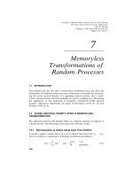
Figure 9.2 Time record of equivalent noise at amplifier input.
convenience, the subscript is removed and power spectral densities are written
as G( f ). Further, the systems are assumed to be such that the fundamental

results, as given by Theorems 8.1 and 8.6, are valid.
9.1.2 The Effect of Noise
In electronic devices, noise is a consequence of charge movement at an atomic
level which is random in character. This random behaviour leads, at a macro
level, to unwanted variations in signals. To illustrate this, consider a signal V
1
,
from a signal source, assumed to be sinusoidal and with a resistance R
1
, which
is amplified by a low noise amplifier as illustrated in Figure 9.1. The equivalent
noise signal at the amplifier input for the case of a 1 k source resistance, and
where the noise from this resistance dominates other sources of noise, is shown
in Figure 9.2. A sample rate of 2.048 kSamples/sec has been used, and 200
samples are displayed. The specific details of the amplifier are described in
Howard (1999b). In particular, the amplifier bandwidth is 30 kHz.
INTRODUCTION
257
0.02 0.04 0.06 0.08 0.1
−0.00001
0
0.00001
0.000015
Time (Sec)
Amplitude (Volts)
−0.000015
−5 · 10
−6
5 · 10
−6

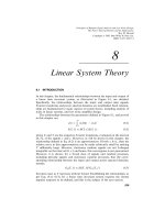
Figure 9.3 Sinusoid of 100 Hz whose amplitude is consistent with a signal-to-noise ratio of 10.
0.02 0.04 0.06 0.08 0.1
−0.00001
0
0.00001
0.000015
Time (Sec)
Amplitude (Volts)
−0.000015
−5 · 10
−6
5 · 10
−6
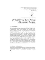
Figure 9.4 100 Hz sinusoidal signal plus noise due to the source resistance and amplifier. The
signal-to-noise ratio is 10.
In Figure 9.3 a 100 Hz sine wave is displayed, whose amplitude is consistent
with a signal-to-noise ratio of 10 assuming the noise waveform of Figure 9.2.
The addition of this 100 Hz sinusoid, and the noise signal of Figure 9.2, is
shown in Figure 9.4 to illustrate the effect of noise corrupting the integrity of
a signal.
For completeness, in Figure 9.5, the power spectral density of the noise
referenced to the amplifier input is shown. In this figure, the power spectral
258
PRINCIPLES OF LOW NOISE ELECTRONIC DESIGN
Figure 9.5 Power spectral density of amplifier noise referenced to the amplifier input.
density has a 1/ f form at low frequencies, and at higher frequencies is constant.
For frequencies greater than 10 Hz, the thermal noise from the resistor
dominates the overall noise.
9.2 GAUSSIAN WHITE NOISE
Gaussian white noise, by which is meant noise whose amplitude distribution

at a set time has a Gaussian density function and whose power spectral density
is flat, that is, white, is the most common type of noise encountered in
electronics. The following section gives a description of a model which gives
rise to such noise. Since the model is consistent with many physical noise
processes it provides insight into why Gaussian white noise is ubiquitous.
9.2.1 A Model for Gaussian White Noise
In many instances, a measured noise waveform is a consequence of the
weighted sum of waveforms from a large number of independent random
processes. For example, the observed randomly varying voltage across a
resistor is due to the independent random thermal motion of many electrons.
In such cases, the observed waveform z, can be modelled according to
z(t) :
+

G
w
G
z
G
(t) z
G
+ E
G
(9.1)
where w
G
is the weighting factor for the ith waveform z
G
, which is from the ith
GAUSSIAN WHITE NOISE

259
Figure 9.6 One waveform from a binary digital random process on the interval [0, 8D].
ensemble E
G
defining the ith random process Z
G
. Here, z is one waveform from
a random process Z which is defined as the weighted summation of the random
processes Z

, ..., Z
+
. Consider the case, where all the random processes Z

, ...,
Z
+
are identical, but independent, signalling random processes and are defined,
on the interval [0, ND], by the ensemble
E
G
:

z
G
(

, ..., 
,
, t) :

,

I

I
(t 9 (k 9 1)D)

I
+ +91, 1,
P[
I
:<1] : 0.5

(9.2)
where the pulse function  is defined according to
(t) :

10- t : D
0 elsewhere
( f ) : D sinc( fD)e\HLD" (9.3)
All waveforms in the ensemble have equal probability, and are binary digital
information signals. One waveform from the ensemble is illustrated in
Figure 9.6.
One outcome of the random process Z, as defined by Eq. (9.1), has the form
illustrated in Figure 9.7 for the case of equal weightings, w
G
: 1, D : 1, and
M : 500. The following subsections show, as the number of waveforms M,
increases, that the amplitude density function approaches that of a Gaussian
function, and that over a restricted frequency range the power spectral density

is flat or ‘‘white’’.
9.2.2 Gaussian Amplitude Distribution
The following, details the reasons why, as the number of waveforms, M,
comprising the random process increases, the amplitude density function
approaches that of a Gaussian function.
The waveform defined by the sum of M equally weighted independent
binary digital waveforms, as per Eq. (9.1), has the following properties: (1)
the amplitudes of the waveform during the intervals [iD,(i ; 1)D), and
[ jD,(j ; 1)D), are independent for i " j; (2) the amplitude A, in any inter-
val [iD,(i ; 1)D] is, for the case where M is even, from the set
260
PRINCIPLES OF LOW NOISE ELECTRONIC DESIGN
0 20 40 60 80 100
−40
−20
0
20
40
60
Amplitude
Time (Sec)
Figure 9.7 Sum of 500 equally weighted, independent, binary digital waveforms where D : 1.
Linear interpolation has been used between the values of the function at integer values of time.
S

: +9M, 9M ; 2, ...,0,..., M 9 2, M,, and M is assumed to be even in
subsequent analysis; (3) at a specific time, the amplitude A, is a consequence
of k ones, and m negative ones where k ; m : M. Thus, A + S

is such that

A : k 9 m. Given A and M, it then follows that
k : (M ; A)/2 m : (M 9 A)/2 (9.4)
Hence, P[A] equals the probability of k : 0.5(A ; M) successes in M out-
comes of a Bernoulli trial. For the case where the probability of success is p,
and the probability of failure is q, it follows that (Papoulis 2002 p. 53)
P[A] :
M!( pI)q+\I
k!(M 9 k)!
:
M!p>+q+\
[0.5(M ; A)]![0.5(M 9 A)]!
(9.5)
To show that P[A] can be approximated by a Gaussian function, consider the
DeMoivre—Laplace theorem (Papoulis 2002 p. 105, Feller 1957 p. 168f ):
Consider M trials of a Bernoulli random process, where the probability of
success is p, and the probability of failure is q. With the definitions
 :
(
Mpq and  : Mp, and the assumption  1, the probability of k
successes in M trials can be approximated according to:
P[k out of M trials] :
M!
k!(M 9 k)!
pIq+\I
e\I\IN
(2
(9.6)
GAUSSIAN WHITE NOISE
261
where a bound on the relative error in this approximation is:


(k 9 )
6
9
(k 9 )
2

k"  (9.7)
For the case being considered, where k : 0.5(A ; M), and p : q : 0.5, it
follows that  : 0.5(M,  : 0.5M, and k 9  : 0.5A. Thus, for 0.25M 1,
the amplitude distribution in any interval [ jD,(j ; 1)D], can be approximated
by the Gaussian form:
P(A) : P

A ; M
2
out of M trials


2e\+
(2M
(9.8)
where a bound on the relative error is

A
12M
9
A
2(M


(9.9)
Note, with the assumptions made, the mean of A is zero, and the rms value of
A is (M. The factor of 2 in Eq. (9.8) arises from the fact that A only takes on
even values. Consistent with this result, many noise sources have a Gaussian
amplitude distribution, and the term Gaussian noise is widely used.
Confirmation, and illustration of this result is shown in Figure 9.8, where
the probability of an amplitude obtained from 1000 repetitions of 100 trials of
a Bernoulli process (possible outcomes are from the set +9100, 998, . . . , 0, . . . ,
100,) is shown. The smooth curve is the Gaussian probability density function
as per Eq. (9.8) with M : 100.
9.2.3 White Power Spectral Density
The power spectral density of the individual random processes comprising Z
are zero mean signaling random processes, as defined by the ensemble of Eq.
(9.2). It then follows, from Theorem 5.1, that the power spectral density of each
of these random processes, on the interval [0, ND], is
G
G
(ND, f ) : r"( f )":
1
r
sinc

f
r

(9.10)
where, r : 1/D, and  is the Fourier transform of the pulse function .AsZ
is the sum of independent random processes with zero means, it follows, from
Theorem 4.6, that the power spectral density of Z is the sum of the weighted
262

PRINCIPLES OF LOW NOISE ELECTRONIC DESIGN
−20 −10 0 10 20
0.02
0.04
0.06
0.08
0.1
Amplitude
Probability
30
Figure 9.8 Probability of an amplitude from the set +9100, 998, . . . , 98, 100, arising from
1000 repetitions of 100 trials of a Bernoulli process. The probabilities agree with the Gaussian
form, as defined in the text.
individual power spectral densities, that is,
G
8
(ND, f ) :
+

G
"w
G
"G
G
(ND, f ) : r"( f )"
+

G
"w
G

"
:
1
r
sinc( f/r)
+

G
"w
G
" (9.11)
This power spectral density is shown in Figure 9.9 for the normalized case of
M : r : 1, and w

: 1. For frequencies lower than r/4, the power spectral
density is approximately constant at a level of M/r, and it is this constant level
that is typically observed from noise sources arising from electron movement.
This is the case because, first, the dominant source of electron movement is,
typically, thermal energy, and electron thermal movement is correlated over an
extremely short time interval. Second, a consequence of this very short
correlation time, is that the rate r, used for modelling purposes, is much higher
than the bandwidth of practical electronic devices. Thus, the common case is
where the noise power spectral density, appears flat for all measurable
frequencies, and the phrase ‘‘white Gaussian noise’’ is appropriate, and is
commonly used.
Note, for processes whose correlation time is very short compared with the
response time of the measurement system (for example, rise time), the power
spectral density will be constant within the bandwidth of the measurement
GAUSSIAN WHITE NOISE
263

0.5 1 1.5 2 2.5 3
0.2
0.4
0.6
0.8
1
G
Z
(ND, f)
Frequency (Hz)
Figure 9.9 Normalized power spectral density as defined by the case where r : M : w

: 1.
system and, consistent with Eq. 9.11, this constancy is independent of the pulse
shape.
9.3 STANDARD NOISE SOURCES
The noise sources commonly encountered in electronics are thermal noise, shot
noise, and 1/ f noise. These are discussed briefly below.
9.3.1 Thermal Noise
Thermal noise is associated with the random movement of electrons, due to the
electrons thermal energy. As a consequence of such electron movement, there
is a net movement of charge, during any interval of time, through an elemental
section of a resistive material as illustrated in Figure 9.10. Such a net movement
of charge, is consistent with a current flow, and as the elemental section has a
defined resistance, the current flow generates an elemental voltage dV. The sum
of the elemental voltages, each of which has a random magnitude, is a random
time varying voltage.
Consistent with such a description, equivalent noise models for a resistor
are shown in Figure 9.11. In this figure, v and i, respectively, are randomly
varying voltage and current sources. These sources are related via Thevenin’s

and Norton’s equivalence statements, namely v(t) : Ri(t), and i(t) : v(t)/R.
Statistical arguments (for example, Reif, 1965 pp. 589—594, Bell, 1960 ch. 3)
can be used to show that the power spectral density of the random processes,
264
PRINCIPLES OF LOW NOISE ELECTRONIC DESIGN
+
−
dV
V
Figure 9.10 Illustration of electron movement in a resistive material.
R
R
i(t)
v(t)
Figure 9.11 Equivalent noise models for a resistor.
which give rise to v and i, respectively, are:
G
4
( f ) :
2h" f "R
eFDI2 9 1
V /Hz (9.12)
G
'
( f ) :
2h" f "
R(eFDI2 9 1)
A/Hz (9.13)
where T is the absolute temperature, k is Boltzmann’s constant (1.38;10\ J/
K), h is Planck’s constant (6.62;10\ J.sec) and R is the resistance of the

material. For frequencies, such that " f ":0.1kT /h 10 Hz (assuming
T : 300K) a Taylor series expansion for the exponential term in these
equations, namely,
eFDI2 1 ; h" f "/kT (9.14)
is valid, and the following approximations hold:
G
4
( f ) 2kT R V /Hz G
'
( f )
2kT
R
A/Hz (9.15)
These equations were derived using the equipartition theorem, and statistical
arguments, by Nyquist in 1928 (Nyquist 1928; Kittel 1958 p. 141; Reif 1965
p. 589; Freeman 1958 p. 117) and are denoted as Nyquist’s theorem. A
STANDARD NOISE SOURCES
265
derivation of these results, based on electron movement, is given in Bucking-
ham 1983 pp. 39—41. Further, these equations are the ones that are nearly
always used in analysis. Note that the power spectral density is ‘‘white’’, that
is, it has a constant level independent of the frequency.
One point to note: In analysis, the Norton, rather than the Thevenin
equivalent noise model for a resistor best facilitates analysis.
9.3.2 Shot Noise
As shown in Section 5.5, shot noise is associated with charge carriers crossing
a barrier, such as that inherent in a PN junction, at random times, but with a
constant average rate. As detailed in Section 5.5.1 the power spectral density,
for all but high frequencies, is given by
G( f ) qI


; I

( f ) A/Hz (9.16)
where q is the electronic charge (1.6;10\ C), and I

is the mean current. Note
that, apart from the impulse at DC, the power spectral density is ‘‘white’’. In
electronic circuits the mean current is associated with circuit bias. As variations
away from the bias state are of interest in analogue electronics, it is usual to
approximate the power spectral density in such circuits, according to
G( f ) qI

A/Hz (9.17)
9.3.3 1/f Noise
As discussed in Section 6.5, the power spectral density of a 1/ f random process
has a power spectral density given by
G( f ) :
k
f ?
(9.18)
where k is a constant, and  determines the slope. Typically,  is close to unity.
At low frequencies, 1/ f noise often dominates other noise sources, and this is
well illustrated in Figure 9.5.
9.4 NOISE MODELS FOR STANDARD ELECTRONIC DEVICES
9.4.1 Passive Components
In an ideal capacitor with an ideal dielectric, all charge is bound, such that
interatomic movement of charge is not possible. Accordingly, an ideal capaci-
tor is noiseless. An ideal inductor is made from material with zero resistance,
and in such a material the voltage created by the thermal motion of electrons

266
PRINCIPLES OF LOW NOISE ELECTRONIC DESIGN
Figure 9.12 (a) Diode symbol. (b) Noise equivalent model for a diode under forward bias. (c)
Noise equivalent model for a diode under reverse bias. I
D
is the DC current flow and C
j
is the
junction capacitance.
is zero. Hence, ideal inductors are noiseless. As discussed above, resistors
exhibit thermal noise, and have either of the noise models shown in Figure 9.11.
Fish (1993 ch. 6) gives a more detailed analysis of noise in passive components.
9.4.2 Active Components
The small signal equivalent noise model for a diode, is shown in Figure 9.12
(Fish, 1993 pp. 126—127). In this figure I
"
is the mean diode current, and the
power spectral density of the small signal equivalent noise source i, is given by
G
"
( f ) : q"I
"
" A/Hz (9.19)
Note, the model of Figure 9.12(c) is also applicable to standard nonavalanche
photodetectors, when they are operated with reverse bias.
The small signal noise equivalent model for a PNP or NPN BJT transistor,
operating in the forward active region, is shown in Figure 9.13 (Fish, 1993
p. 128). The sources i

, i

, and i
!
in this figure, respectively model the thermal
noise in the base due to the base spreading resistance r
@
, which is typically in
the range of 10—500 Ohms (Gray, 2001 p. 32; Fish, 1993 pp. 128—139), the shot
noise of the base current and the collector current shot noise (see Edwards,
2000). The respective power spectral densities of these noise sources are
G

( f ) : 2kT /r
@
A/Hz (9.20)
G

( f ) : qI

A/Hz G
!
( f ) : qI
!
A/Hz (9.21)
In analysis, it is usual to neglect r
M
as, typically, it is in parallel with a much
lower value load resistance.
The small signal noise equivalent model for a NMOS or PMOS MOSFET,
with the source connected to the substrate, and a N or P channel JFET, when

they are operating in the saturation region, is shown in Figure 9.14 (for
NOISE MODELS FOR STANDARD ELECTRONIC DEVICES
267
C
π
r
π
C
µ
+
−
B
E
V
NPN
PNP
I
C
I
C
I
B
I
B
i
BB
(t)
r
b
i

B
(t)
g
m
V
i
C
(t)
r
o
C
Figure 9.13 Small signal equivalent noise model for a NPN or PNP BJT operating in the
forward active region.
C
gs
+
−
G
V
D
S
NMOS
PMOS
I
D
I
D
I
G
I

G
C
gd
i
G
(t)
g
m
V
i
D
(t)
r
o
Figure 9.14 Small signal equivalent noise model for a PMOS or NMOS MOSFET, or a N or
P channel JFET, operating in the saturation region.
example, Fish, 1993 p. 140; Levinzon, 2000; Howard, 1987). In this figure, the
noise sources i
%
and i
"
, respectively, account for the noise at the gate, which is
due to the gate leakage current and the induced noise in the gate due to
thermal noise in the channel, and the thermal noise in the channel. The
respective power spectral densities of these sources are
G
%
( f ) : q"I
%
" ; 2kT 


(2 fC
EQ
)/g
K
A/Hz (9.22)
G
"
( f ) : 2kT Pg
K
A/Hz (9.23)
In these equations, 

is a constant with a value of around 0.25 for JFETs, and
0.1 for MOSFETS (Fish, 1993 p. 141). P is a constant with a theoretical value
of 0.7, but practical values can be higher (Howard, 1987; Muoi, 1984; Ogawa,
1981). I
%
is the gate leakage current which, typically, is in the pA range. As
with a BJT, it is usual to neglect r
M
in analysis.
268
PRINCIPLES OF LOW NOISE ELECTRONIC DESIGN
h ↔ H
G
X
x ∈E
X
G

Y
y ∈E
Y
Figure 9.15 Schematic diagram of a linear system.
9.5 NOISE ANALYSIS FOR LINEAR TIME INVARIANT SYSTEMS
The following discussion relates to analysis of noise in linear time invariant
systems — linear electronic systems are an important subset of such systems.
9.5.1 Background and Assumptions
A schematic diagram of a linear system is shown in Figure 9.15. With the
assumption that the results of Theorems 8.1 and 8.6 are valid, the relationship
between the input and output power spectral densities, on the infinite interval
[0, -], or a sufficiently long interval relative to the impulse response time of
the system, is given by
G
7
( f ) : "H( f )"G
6
( f ) (9.24)
In this diagram, the input random process X is defined by the ensemble E
6
,
and the output random process Y is defined by the ensemble E
7
.
9.5.1.1 Transfer Functions and Notation Analysis of electronic circuits
is usually performed through use of Laplace transforms (for example, Chua,
1987 ch. 10). Such analysis yields a relationship, assuming appropriate excita-
tion, between the Laplace transform of the ith and jth node voltage or current,
of the form V
H

(s)/V
G
(s) : L
GH
(s). If the time domain input at the ith node, v
G
(t),
is an ‘‘impulse,’’ then V
G
(s) : 1 and, hence, the output signal v
H
(t) is the impulse
response, whose Laplace transform is given by L
GH
(s). In the subsequent text,
the following notation will be used: L
GH
is denoted the Laplace transfer function,
while H
GH
, which is the Fourier transform of the impulse response, is simply
denoted the transfer function. From the definitions for the Laplace and Fourier
transform, it follows that the relationship between these transfer functions is
H
GH
( f ) : L
GH
( j2f ) (9.25)
The Fourier transform H
GH

, is guaranteed to exist if the impulse response h
GH
,is
such that h
GH
+ L [0, -]. Similarly, the Laplace transform L
GH
, will exist, with a
region of convergence including the imaginary axis, when h
GH
+ L [0, -].
Finally, in circuit analysis, it is usual to omit the argument s from Laplace
transformed functions. To distinguish between a time function, and its asso-
ciated Laplace transform, capital letters are used for the latter, while lowercase
letters are used for the former.
NOISE ANALYSIS FOR LINEAR TIME INVARIANT SYSTEMS
269
w
M
(t)
Linear Circuit
w
0
(t)
w
1
(t)
w
N
(t)w

i
(t)
Figure 9.16 Schematic diagram of a linear system with N noise sources.
9.5.2 Input Equivalent Noise — Individual Case
The definition of the input equivalent noise of a linear system, is fundamental
to low noise amplifier design. The following is a brief summary: When all
components in a linear circuit have been replaced by their equivalent circuit
models, including appropriate models for noise sources, the circuit, as illus-
trated in Figure 9.16, results.
In this figure w

and w
+
respectively, are the input and output signals of
the circuit, and w

, ..., w
,
are signals from the ensembles defining the N noise
sources in the circuit. The Laplace transform of these signals are, respectively,
denoted by W

, W

, ..., W
,
, W
+
. The transfer function between the source and
the output, denoted H

+
, is defined according to
H
+
( f ) : L
+
( j2f ) :
W
+
( j2f )
W

( j2f )

U

B U

U
,

(9.26)
where,  denotes the Dirac delta function, and it is assumed that w
+
+ L [0, -],
when w

: , such that, the results of Theorem 8.3 are valid. Similarly, the
transfer functions H
+

, ..., H
,+
are defined as the transfer functions that
relate the noise sources w

, ..., w
,
to the amplifier output, and are defined as
H
G+
( f ) : L
G+
( j2f ) :
W
+
( j2f )
W
G
( j2f )

U
G
BU

U

U
G\
U
G>

U
,

(9.27)
It is usual, when quantifying the noise performance of an amplifier, to refer the
noise to the amplifier input in order that it is independent of the amplifier gain.
To achieve this, it is necessary to define an input equivalent noise source for
each of the noise sources in the amplifier. By definition, the input equivalent
noise source, denoted w
CG
, for the ith noise source w
G
, is the equivalent noise
source at the amplifier input that produces the same level of output noise as
w
G
. That is, by definition, w
CG
guarantees the equivalence of the circuits shown
in Figures 9.17 and 9.18, as far as the output noise is concerned.
Assume, for the circuit shown in Figure 9.17, that either, or both the source
w

, and the ith noise source w
G
, have zero mean, and the source is independent
of the ith noise source. It then follows, from Theorem 8.7, that the output
270
PRINCIPLES OF LOW NOISE ELECTRONIC DESIGN
w

0
(t)
Linear
Circuit
w
i
(t) w
M
(t)
Figure 9.17 Noise model for ith noise source.
Noiseless
Linear Circuit
w
0
(t) w
ei
(t)
w
M
(t)
Figure 9.18 Equivalent noise model, as far as the output node is concerned, for the ith noise
source.
power spectral density, G
+
, due to w

and w
G
is
G

+
( f ) : "H
+
( f )"G

( f ) ; "H
G+
( f )"G
G
( f ) (9.28)
where G

and G
G
, respectively, are the power spectral densities of w

and w
G
.
For the circuit shown in Figure 9.18, the output power spectral density due to
the noise sources w

and w
CG
,is
G
+
( f ) : "H
+
( f )"G


( f ) ; "H
+
( f )"G
CG
( f ) (9.29)
where G
CG
is the power spectral density of the input equivalent source w
CG
.A
comparison of Eqs. (9.28) and (9.29) shows that these two circuits are
equivalent, in terms of the output power spectral density, when
"H
+
( f )"G
CG
( f ) : "H
G+
( f )"G
G
( f ) (9.30)
Thus, the power spectral density of the input equivalent noise source associated
with the ith noise source is
G
CG
( f ) :
"H
G+
( f )"

"H
+
( f )"
G
G
( f ) : "H
CO
G+
( f )"G
G
( f ) (9.31)
where H
CO
G+
( f ) : H
G+
( f )/H
+
( f ) is the transfer function between the ith noise
source, w
G
, and the associated input equivalent noise source w
CG
.
NOISE ANALYSIS FOR LINEAR TIME INVARIANT SYSTEMS
271
9.5.3 Input Equivalent Noise ----— General Case
For the general case of determining the input equivalent noise of all the N
noise sources, the approach is to, first, establish the input equivalent signal and,
then, evaluate its power spectral density. The details are as follows: the N noise

signals generate an output signal according to
w
+
(t) :

R

w

()h
+
(t 9 )d ; ···;

R

w
,
()h
,+
(t 9 )d (9.32)
where, h
+
, ..., h
,+
are the impulse responses of the systems between w
G
and
w
K
for i + +1, ..., N,. From Theorem 8.3 it follows that

W
+
(s) : W

(s)L
+
(s) ; ···; W
,
(s)L
,+
(s) Re[s] 9 0 (9.33)
where, L
G+
is the Laplace transform of h
G+
, and the noise signals are assumed
not to have exponential increase, which is the usual case. An equivalent input
signal, w
CO
, whose Laplace transform is W
CO
, will result in an output signal with
the same Laplace transform when
W
CO
(s)L
+
(s) : W

(s)L

+
(s) ; ···; W
,
(s)L
,+
(s) Re[s] 9 0 (9.34)
Thus, provided L
+
(s) " 0, it is the case that
W
CO
(s) :
,

G
W
CG
(s) :
,

G
W
G
(s)L
G+
(s)
L
+
(s)
Re[s] 9 0 (9.35)

where W
CG
is the Laplace transform of the ith input equivalent signal associated
with w
G
. Consistent with this result, an equivalent model for the input
equivalent noise is as shown in Figure 9.19. The ith transfer function in this
figure, from Eq. (9.35), is given by
H
CO
G+
( f ) :
L
G+
( j2f )
L
+
( j2f )
:
H
G+
( f )
H
+
( f )
H
+
( f ) " 0 (9.36)
where L
G+

(s) and L
+
(s) are validly defined when Re[s] : 0, as assumed in
Eqs. (9.26) and (9.27). The following theorem states the power spectral density
of the input equivalent noise random process.
T 9.1 P S D  I E N For
independent noise sources with zero means, the amplifier input equivalent power
spectral density, denoted G
CO
( f ), is the sum of the individual input equivalent
power spectral densities, that is,
G
CO
( f ) :
,

G
G
CG
( f ) :
,

G
"H
CO
G+
( f )"G
G
( f ) :
,


G

H
G+
( f )
H
+
( f )


G
G
( f ) (9.37)
where G
G
and G
CG
, respectively, are the power spectral density, and the input
equivalent power spectral density, of the ith noise source. For the general case,
272
PRINCIPLES OF LOW NOISE ELECTRONIC DESIGN