Tài liệu Nguyên tắc phân tích tín hiệu ngẫu nhiên và thiết kế tiếng ồn thấp P3 pptx

3
The Power
Spectral Density
3.1 INTRODUCTION
The power spectral density is widely used to characterize random processes in
electronic and communication systems. One common application of the power
spectral density is to characterize the noise in a system. From such a
characterization the noise power, and hence, the system signal to noise ratio,
can be evaluated. This chapter gives a detailed justification of the two distinct,
but equivalent ways of defining the power spectral density. The first is via
decomposition, as given by the Fourier transform, of signals comprising
the random process; the second is through the Fourier transform of the
time averaged autocorrelation function of waveforms comprising the ran-
dom process. The first approach is used in later chapters and facilitates analysis
to a greater degree than the second. Finally, the relationship between the
power spectral density and autocorrelation function, as stated by the Wiener—
Khintchine theorem, is justified. A brief historical account of the development
of the theory underlying the power spectral density can be found in Gardner
(1988 pp. 12f ).
3.1.1 Relative Power Measures
In the following sections, the concepts of signal power and signal power
spectral density are introduced and used. Strictly speaking, the concepts are
that of relative signal power and relative signal power spectral density, as
signals typically have units that lead to relative, not absolute, power measures.
To simplify terminology, the word ‘‘relative’’ is dropped. The best justification
for the use of relative power measures, is the signal to noise ratio which is
defined as the signal power divided by the noise power. Provided both the
59
Principles of Random Signal Analysis and Low Noise Design:
The Power Spectral Density and Its Applications.
Roy M. Howard

Copyright
¶
2002 John Wiley & Sons, Inc.
ISBN: 0-471-22617-3
signal and noise have the same units, for example, watts or volts squared, it
does not matter whether relative or absolute power measures are used. Further,
in many electronic circuit applications a relative power measure is appropriate
as it is current and voltage levels, not power levels, that are of interest.
3.2 DEFINITION
The approach detailed in this section is consistent with that of Priestley (1981
ch. 4.3—4.8), Jenkins (1968 ch. 6), and Peebles (1993 ch. 7).
3.2.1 Characteristics of a Power Spectral Density
A power spectral density function, G, based on the standard sinusoidal or
complex exponential basis set should have the following characteristics. First,
to facilitate analysis it should be a continuous signal. Second, it should have
the interpretation that G( f
V
) is directly proportional to the power in the
sinusoidal components of the signal with a frequency of f
V
Hz. Third, this
proportionality should be such that the integral of the power spectral density
over all possible frequencies equals the average signal power denoted P

, that is,
P

:



\
G( f ) df (3.1)
This last requirement is consistent with the sum of the power in the constituent
waveforms equaling the total average power. In summary, a power spectral
density function G, should be such that
(1) G is a continuous function.
(2) G( f
V
) is proportional to the power of the constituent sinusoidal signals
with frequency f
V
.
(3) P

: 

\
G( f ) df.
The following subsections give details of a power spectral density function that
satisfies these three conditions or requirements.
3.2.2 Power Spectral Density of a Single Waveform
A natural basis for the power spectral density is the average power of a signal.
For an interval [0, T ] the average power of a signal x, by definition, is
P

(T ) :
1
T

2


"x(t)" dt (3.2)
Assume that x is either piecewise smooth or of bounded variation. It then
60
THE POWER SPECTRAL DENSITY
2
2
2
2
2
−3f
o
−2f
o
−f
o
f
o
2f
o
3f
o
2
f
c
−3
c
−2
c
−1

c
0
c
1
c
2
c
3
2
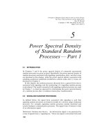
Figure 3.1 Display of power in sinusoidal components of a signal.
−f
o
f
o
−2f
o
2f
o
−3f
o
3f
o
G(T, f )
f
X(T,0)
2
T
c
0
2

f
o
=
X(T, −2f
o
)
T
2
c
−2
2
f
o
=
X(T, 2f
o
)
T
2
c
2
2
f
o
=
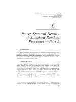
Figure 3.2 A power spectral density function. T he shaded areas equal the power associated
with sinusoidal components that have a frequency of 2f
o
Hz.
follows, from substitution of the Fourier series for the signal x [see Eq. (2.126)]

into this equation, that
P

(T ) : "a

";0.5


G
"a
G
";"b
G
":


G\
"c
G
":


G\
"X(T, if
M
)"
T 
(3.3)
where the last relationship follows from Eq. (2.137). As per Eq. (2.131), the
power associated with signal components with a frequency of if

M
Hz, namely,
a
G
cos(2if
M
t) and b
G
sin(2if
M
t), is given by "c
\G
";"c
G
":("a
G
";"b
G
")/2. Con-
sistent with this result, Figure 3.1 represents one way to display the power in
the sinusoidal components of a single waveform, subject to the interpretation
that the power in the sinusoidal components with a frequency of if
M
is the sum
of the values defined by the graph at frequencies of 9if
M
and if
M
Hz.
Note, for a real signal "c

\G
":"c
G
" and the display is symmetric with respect
to the vertical axis.
A problem with such a display is that the integral of the function defined by
the graph is zero. To overcome this problem an alternative display, based on
the relationship c
G
: X(T, if
M
)/T, can be constructed as shown in Figure 3.2.
DEFINITION
61
With such a graph the area under the defined function, by construction, equals
the average signal power.
The display in Figure 3.2 is consistent with writing the average power in the
form,
P

(T ) :


G\
"X(T, if
M
)"
T 
(3.4)
The interpretation of the graph in Figure 3.2 is as follows: The area under each

pair of levels of the graph associated with the frequencies 9if
M
and if
M
, equals
the power in the sinusoidal waveforms with a frequency if
M
. Consistent with this
graph, the power spectral density function, G, can be defined as
G(T, f ) :
"X(T, if
M
)"
T
if
M
9
f
M
2
- f : if
M
;
f
M
2
(3.5)
or, more generally, according to
G(T, f ) :
1

T

X

T,
f ; f
M
/2
f
M
f
M


9- : f : - (3.6)
With such a definition it follows that
P

(T ) :


\
G(T, f ) df (3.7)
which is the third requirement of a power spectral density function.
Such a power spectral density function G, satisfies requirements (2) and (3)
but is not a continuous function. Obtaining a continuous function for the
power spectral density is discussed in the next subsection.
3.2.3 A Continuous Power Spectral Density Function
The basis for obtaining a continuous waveform for the power spectral density
is Parseval’s relationship (Theorem 2.31):


2

"x(t)" dt :


\
"X(T, f )" df (3.8)
Scaling both integrals by T yields
P

(T ) :
1
T

2

"x(t)" dt :


\
"X(T, f )"
T
df :


\
G(T, f ) df (3.9)
62
THE POWER SPECTRAL DENSITY

f
x
f
2
G( T,f ) = X (T,f ) /T
G( T,f
x
)
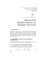
Figure 3.3 Continuous power spectral density function based on Parseval’s relationship.
and a power spectral density function G, as per the following definition:
D:P S D The power spectral density of a signal
x, evaluated on the interval [0, T ], is defined according to
G(T, f ) :
"X(T, f )"
T
(3.10)
This power spectral density function is commonly called the periodogram (see
Gardner, 1988 p. 13) or sample spectral density (Jenkins, 1968 p. 211; Parzen,
1962 p. 109).
The power spectral density function, as defined by Eq. (3.10), has the form
shown in Figure 3.3 and it remains to show that it satisfies the three
requirements of a power spectral density function. To this end note, first, that
the integral of the power spectral density, by construction, equals the total
power. Second, the power spectral density is a continuous function as stated
by the following theorem (Champeney, 1987 p. 60).
T 3.1. C  P S D If x + L [0, T ] then
the power spectral density function G, defined by Eq. (3.10), is continuous with
respect to f for f + R.
Proof. This result can be proved by first proving that X(T, f ) is continuous
with respect to f + R when x + L [0, T ]. The proof is straightforward and is

omitted.
Third, the last requirement of a power spectral density function is that
G(T, f
V
) should be proportional to the power in the constituent sinusoidal
components that have a frequency of f
V
Hz. This is not obviously the case,
because a Fourier series decomposition on the interval [0, T ] only yields
sinusoids with frequencies f
M
,2f
M
, ..., where f
M
: 1/T. It may well be the case
that f
V
is not an integer multiple of f
M
. This issue is discussed in the following
subsection.
DEFINITION
63
f
−(i + 1)f
o
−(i − 1)f
o
−if

o
(i − 1)f
o
(i + 1)f
o
f
x
= if
o
=
f
o
G(T, f ) =
2
T
X(T, f )
2
T
X(T, if
o
)
2
f
o
c
i
Figure 3.4 Step approximation to power spectral density function. The area under the two
levels associated with f :9if
o
and f : if

o
equals the power in the sinusoidal components of the
signal with a frequency of if
o
Hz.
3.2.3.1 Interpretation of Continuous Power Spectral Density Function
As a Fourier series decomposition of a signal on an interval [0, T ] yields
sinusoidal components with frequencies f
M
,2f
M
, ...it is reasonable to conclude
that G(T, f
V
) should only be interpreted for f
V
: if
M
, i + Z>. The problem then
is, how to interpret G(T, if
M
) for some integer value of i. The interpretation is
given in the following theorem.
T 3.2. I  P S D If x + L [0, T ],
and the power spectral density of x is defined according to
G(T, f ) :
"X(T, f )"
T
f
M

:
1
T
(3.11)
then the average power in the sinusoidal components of x with a frequency if
M
,
and on the interval [0, T ], is given by
"c
\G
";"c
G
": f
M
[G(T, 9if
M
) ; G(T, if
M
)] i + Z>
(3.12)
"c

": f
M
G(T,0) i : 0
Proof. Using the relationship c
G
: X(T, if
M
)/T a step approximation to G can

be defined, as shown in Figure 3.4 and consistent with that shown in Figure
3.2. With such a step approximation the area under each pair of levels with
width f
M
, centered at <if
M
and with respective heights "X(T, 9if
M
)"/T and
"X(T, if
M
)"/T, equals "c
\G
";"c
G
", and hence, the power in the sinusoidal
components with a frequency of if
M
Hz.
This theorem states that the power in the mean of a signal is given by
f
M
G(T,0). To confirm this, note that the mean 
V
of the signal x on [0, T ]is
given by

V
(T ) :
1

T

2

x(t) dt :
X(T,0)
T
(3.13)
64
THE POWER SPECTRAL DENSITY
and this implies the following relationships:
P

I
V
(T ) :
1
T

2

"
V
" dt : "
V
":
"X(T,0)"
T 
: "c


": f
M
G(T,0) (3.14)
3.2.3.2 Power as Area Under the Power Spectral Density Graph The
power in the sinusoidal components with a frequency if
M
can be approximated
by the integral
"c
\G
";"c
G
"

\GD
M
>D
M

\GD
M
\D
M

G(T, f ) df ;

GD
M
>D
M


GD
M
\D
M

G(T, f ) df
(3.15)
: 2

GD
M
>D
M

GD
M
\D
M

G(T, f ) df
where the last equality in this equation only applies for real signals. How
accurate this approximation is depends on the nature of the signal under
consideration, and hence, G. The following example illustrates this point.
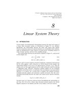
3.2.3.3 Example — Power Spectral Density of a Sinusoid Consider a
sinusoidal signal A sin(2f
A
t) on the interval [0, T ]. From Eq. (3.10) it follows,
after standard analysis, that the power spectral density can be written as
G(T, f ) :

AT
4

sinc

N

f
f
A
9 1

; sinc

N

f
f
A
; 1

9 2 sinc

N

f
f
A
9 1


sinc

N

f
f
A
; 1

(3.16)
where T : NT
A
with T
A
: 1/ f
A
. This power spectral density is shown in Figure
3.5 for the case where A : 1, T : 1/f
M
: 1, and f
A
: 4. Note that G(T, if
M
) : 0
as expected, except for the case when if
M
: f
A
. However, it is clearly evident
from this figure that

"c
\G
";"c
G
":2"c
G
":0 " 2

GD
M
>D
M

GD
M
\D
M

G(T, f ) df

i : 1, 2, 3, 5, 6, ...
f
M
: 1
(3.17)
3.3 PROPERTIES
The following subsections detail basic properties of the defined power spectral
density function.
PROPERTIES
65

0 2 4 6 8
0
0.05
0.1
0.15
0.2
0.25
G(T, f )
Frequency (Hz)
Figure 3.5 Power spectral density of a sinusoid with a frequency of 4 Hz, an amplitude of
unity, and evaluated on a 1 sec interval (f
o
: 1).
3.3.1 Symmetry in Power Spectral Density
For the case where x is real it follows that G is an even function with respect
to f, that is, G(T, 9 f ) : G(T, f ). This result follows from Eq. (2.136) which
states:
X(T, 9 f ) : X*(T, f )
3.3.2 Resolution in Power Spectral Density
For a measurement interval of T seconds, the frequency resolution in the
power spectral density is f
M
: 1/T. Clearly, as T increases the resolution
increases. In fact, for any resolution f in frequency, there exists an interval
[0, T ], where T : 1/f, such that the rectangular areas of width f, centered
at the frequencies 9 f
V
and f
V
and with respective heights of G(T, 9f

V
) and
G(T, f
V
), equal the power in the sinusoidal components of the signal with a
frequency f
V
. The assumption here is that the frequency f
V
is some integer
multiple of the resolution f. This result is illustrated in Figure 3.4 provided f
M
is interpreted as f. Note that, in general, G(T, f ) will vary with T.
3.3.3 Integrability of Power Spectral Density
An important property of the power spectral density function G, is that, in
general, it is integrable.
66
THE POWER SPECTRAL DENSITY
T 3.3. I  P S D If x + L [0, T ]
then G + L .
Proof. Given x + L [0, T ] it follows from Parseval’s relationship that


\
"X(T, f )" df
is finite which implies the integrability of G.
3.3.4 Power Spectral Density on Infinite Interval
Taking the limit as T tends toward infinity of the average power on the interval
[0, T ] yields a definition for the average signal power on the interval (0, -),
denoted P



, that is,
P


: lim
2
1
T

2

"x(t)" dt : lim
2


\
"X(T, f )"
T
df : lim
2


\
G(T, f ) df
(3.18)
If it is possible to interchange the order of integration and limit operations in
the last equation, then P



can be rewritten as
P


: lim
2


\
G(T, f ) df :


\
lim
2
G(T, f ) df (3.19)
and a power spectral density function G

, for the interval [0, -] can be
defined according to the following definition.
D:P S D  I I
G

( f ) : lim
2
G(T, f ) (3.20)
Note, the standard results that dictate whether it is possible to interchange the
order of integration and limit operations are the Dominated and Monotone
convergence theorems (Theorems 2.23 and 2.24).

3.4 RANDOM PROCESSES
Consider a random process X with ensemble
E
6
: +x: S
6
; [0, T ] ; C, (3.21)
RANDOM PROCESSES
67
and associated signal probabilities
P[x(i, t)] : P[x
G
(t)] : p
G
S
6
3 Z> countable case
P[x(, t)"
HZH
M
H
M
>BH
] : f
6
(
M
) d S
6
3 R uncountable case

(3.22)
The average power in an individual waveform from the ensemble evaluated
over the interval [0, T ]is
P

(, T ) :
1
T

2

"x(, t)" dt (3.23)
For the countable case it is convenient to use a subscript rather than an
argument according to x(i, T ) : x
G
(T ) and P

(i, T ) : P

G
(T ).
The probabilities defined in Eq. (3.22) are the ‘‘natural’’ weighting factor to
use in determining the average signal power according to
P

(T ) :


G
p

G
P

G
(T ) :


G
p
G
1
T

2

"x
G
(t)" dt countable case (3.24)
P

(T ) :


\
P

(, T ) f
6
() d
:



\

1
T

2

"x(, t)" dt

f
6
() d uncountable case (3.25)
Provided Parseval’s relationship can be applied, and the order of summa-
tion/integration and integration can be interchanged, then the average signal
power can be written as
P

(T ) :


\
1
T


G
p
G

"X
G
(T, f )" df :


\
G(T, f ) df countable case (3.26)
P

(T ) :


\

1
T


\
"X(, T, f )"f
6
() d

df
:


\
G(T, f ) df uncountable case
(3.27)

where
X
G
(T, f ) :

2

x
G
(t)e\HLDR dt X(, T, f ) :

2

x(, t)e\HLDR dt (3.28)
and G: R ; R is the power spectral density function for the random process
X, on the interval [0, T ], and defined according to:
68
THE POWER SPECTRAL DENSITY
D:P S D  F I
G(T, f ):

1
T


G
p
G
"X
G

(T, f )":


G
p
G
G
G
(T, f ) countable case
1
T


\
"X(, T, f )"f
6
() d:


\
G(, T, f ) f
6
() d uncountable case
(3.29)
where G
G
(T, f ) and G(, T, f ), respectively, are the power spectral densities for
the ith and th signals in the countable and uncountable ensembles.
Clearly, the power spectral density of a random process is the weighted
average of the power spectral density of individual signals in the ensemble.

3.4.1 Power Spectral Density on Infinite Interval
The countable case is considered here. The analysis for the uncountable case
follows in an analogous manner.
The average power of the random process on the interval [0, -], denoted
P


, by definition, is the weighted sum of the individual signal powers
comprising the random process X as T tends towards infinity, that is,
P


:


G
p
G
lim
2
P

G
(T ) :


G
p
G
lim

2
1
T

2

"x
G
(t)" dt (3.30)
By using Parseval’s relationship, interchanging the order of the summation and
limit operations, and then interchanging the order of the summation and
integration, the average power can be written according to
P


: lim
2


\
1
T


G
p
G
"X
G
(T, f )" df : lim

2


\
G(T, f ) df (3.31)
If it is possible to interchange the order of the limit and integral operations in
this last equation, then the average power can be written as
P


:


\
lim
2
G(T, f ) df :


\
G

( f ) df (3.32)
where G

: R ; R is the power spectral density for the random process on the
infinite interval (0, -) and defined as:
D:P S D  I I
G


( f ) : lim
2
G(T, f ) (3.33)
RANDOM PROCESSES
69
–1
1
t
2D
6D
8D
D
p(t)
4D
x(1, −1, −1, 1, –1, 1, 1, –1, t)
Figure 3.6 One waveform from a binary digital random process on the interval [0, 8D].
3.4.2 Example — PSD of Binary Digital Random Process
Consider a binary digital random process X, defined by either a pulse p or its
negative 9p in each interval of D sec. On the interval [0, ND] the ensemble
for this random process is
E
6
:

x(

, ..., 
,
, t) :
,


I

I
p(t 9 (k 9 1)D), 
I
+ +91, 1,

(3.34)
One of the 2, possible waveforms in this ensemble is shown in Figure 3.6 for
the case of a rectangular pulse function of duration D/2 sec. For the case where
the pulses are independent from one interval of D sec to the next, the
probability of a signal from the ensemble is
P[x(

, ..., 
,
, t)] : P[

, ..., 
,
] : P[

]P[

] % P[
,
] (3.35)
For the case where the probability of a pulse p is equal to the probability of
9p, that is, P[

I
: 1] : P[
I
:91] : 0.5, then the probability of any signal
from the ensemble is 1/2,. It follows from the definition of the power spectral
density function, that the power spectral density of X, evaluated on the interval
[0, ND], is given by
G
6
(ND, f ) :
1
ND

A

% 
A
,
1
2,
"X(

, ..., 
,
, ND, f )" 
G
+ +<1, (3.36)
To evaluate the power spectral density, the assumption is made that the pulse
function is zero outside the interval [0, D]. With this assumption, first note that
"X(


, ..., 
,
, ND, f )":
,

G
,

I

G

I
"P( f )"e\HLDG\"De HLDI\"D
:
,

G
"P( f )";
,

G
,

I
I$G

G


I
"P( f )"e\HLDG\I"D (3.37)
70
THE POWER SPECTRAL DENSITY
0.01
0.05
0.1
0.5 1
0.01
0.02
0.05
0.1
0.2
0.5
1
W = D/2 W = D
Frequency (Hz)
G
X
(ND, f )
Figure 3.7 Power spectral density of binary digital random process for the case where D : 1.
where P is the Fourier transform of p. Next, note that substitution of Eq. (3.37)
into Eq. (3.36) and interchanging the order of summation yields, for the second
term:
1
ND2,
,

G
,


I
I$G
"P( f )"e\HLDG\I"D 
A

% 
A
,

G

I
(3.38)
This summation is zero as 
G
+ +<1, and 
G
is independent of 
I
for i " k. Hence,
G
6
(ND, f ) : r"P( f )" (3.39)
where, r : 1/D. Note that the power spectral density in independent of the
interval being considered. This is due to the fact that the pulse function is zero
outside the interval [0, D]. The power spectral density is plotted in Figure 3.7
for the case where the pulse function is rectangular, that is,
p(t) :


10- t : W
0 elsewhere
P( f ) : W sinc( fW)e\HLD5
0 : W - D
(3.40)
3.4.3 Miscellaneous Issues
3.4.3.1 Nonstationary Random Processes The definition for the power
spectral density [see Eq. (3.29)] is valid for single waveforms, stationary
random processes, and nonstationary random processes, as it is based on
RANDOM PROCESSES
71