Tài liệu Độ tin cậy của hệ thống máy tính và mạng P5 docx

5
SOFTWARE RELIABILITY AND
RECOVERY TECHNIQUES
Reliability of Computer Systems and Networks: Fault Tolerance, Analysis, and Design
Martin L. Shooman
Copyright 
2002
John Wiley & Sons, Inc.
ISBNs:
0
-
471
-
29342
-
3
(Hardback);
0
-
471
-
22460
-X (Electronic)
202
5
.
1
INTRODUCTION
The general approach in this book is to treat reliability as a system problem
and to decompose the system into a hierarchy of related subsystems or com-
ponents. The reliability of the entire system is related to the reliability of the

components by some sort of structure function in which the components may
fail independently or in a dependent manner. The discussion that follows will
make it abundantly clear that software is a major “component” of the system
reliability,
1
R. The reason that a separate chapter is devoted to software reli-
ability is that the probabilistic models used for software differ from those used
for hardware; moreover, hardware and software (and human) reliability can be
combined only at a very high system level. (Section
5
.
8
.
5
discusses a macro-
software reliability model that allows hardware and software to be combined at
a lower level.) Specifically, if the hardware, software, and human failures are
independent (often, this is not the case), one can express the system reliabil-
ity, R
SY
, as the product of the hardware reliability, R
H
, the software reliability,
R
S
, and the human operator reliability, R
O
. Thus, if independence holds, one
can model the reliability of the various factors separately and combine them:
R

SY

R
H
× R
S
× R
O
[Shooman,
1983
, pp.
351
–
353
].
This chapter will develop models that can be used for the software reliabil-
ity. These models are built upon the principles of continuous random variables
1
Another important “component” of system reliability is human reliability if an operator is
involved in any control, monitoring, input, or similar task. A discussion of human reliability
models is beyond the scope of this book; the reader is referred to Dougherty and Fragola [
1988
].
INTRODUCTION
203
developed in Appendix A, Sections A
6
and A
7
, and Appendix B, Section B

3
;
the reader may wish to review these concepts while reading this chapter.
Clearly every system that involves a digital computer also includes a signif-
icant amount of software used to control system operation. It is hard to think
of a modern business system, such as that used for information, transportation,
communication, or government, that is not heavily computer-dependent. The
microelectronics revolution has produced microprocessors and memory chips
that are so cheap and powerful that they can be included in many commercial
products. For example, a
1999
luxury car model contained
20
–
40
micropro-
cessors (depending on which options were installed), and several models used
local area networks to channel the data between sensors, microprocessors, dis-
plays, and target devices [New York Times, August
27
,
1998
]. Consumer prod-
ucts such as telephones, washing machines, and microwave ovens use a huge
number of embedded microcomponents. In
1997
,
100
million microprocessors
were sold, but this was eclipsed by the sale of

4
.
6
billion embedded microcom-
ponents. Associated with each microprocessor or microcomponent is memory,
a set of instructions, and a set of programs [Pollack,
1999
].
5
.
1
.
1
Definition of Software Reliability
One can define software engineering as the body of engineering and manage-
ment technologies used to develop quality, cost-effective, schedule-meeting soft-
ware. Software reliability measurement and estimation is one such technology
that can be defined as the measurement and prediction of the probability that the
software will perform its intended function (according to specifications) without
error for a given period of time. Oftentimes, the design, programming, and test-
ing techniques that contribute to high software reliability are included; however,
we consider these techniques as part of the design process for the development
of reliable software. Software reliability complements reliable software; both, in
fact, are important topics within the discipline of software engineering. Software
recovery is a set of fail-safe design techniques for ensuring that if some serious
error should crash the program, the computer will automatically recover to reini-
tialize and restart its program. The software succeeds during software recovery
if no crucial data is lost, or if an operational calamity occurs, but the recovery
transforms a total failure into a benign or at most a troubling, nonfatal “hiccup.”
5

.
1
.
2
Probabilistic Nature of Software Reliability
On first consideration, it seems that the outcome of a computer program is
a deterministic rather than a probabilistic event. Thus one might say that the
output of a computer program is not a random result. In defining the concept
of a random variable, Cramer [Chapter
13
,
1991
] talks about spinning a coin as
an experiment and the outcome (heads or tails) as the event. If we can control
all aspects of the spinning and repeat it each time, the result will always be
the same; however, such control needs to be so precise that it is practically
204
SOFTWARE RELIABILITY AND RECOVERY TECHNIQUES
impossible to repeat the experiment in an identical manner. Thus the event
(heads or tails) is a random variable. The remainder of this section develops
a similar argument for software reliability where the random element in the
software is the changing set of inputs.
Our discussion of the probabilistic nature of software begins with an exam-
ple. Suppose that we write a computer program to solve the roots r
1
and r
2
of a quadratic equation, Ax
2
+ Bx + C


0
. If we enter the values
1
,
5
, and
6
for A, B, and C, respectively, the roots will be r
1

−
2
and r
2

−
3
. A sin-
gle test of the software with these inputs confirms the expected results. Exact
repetition of this experiment with the same values of A, B, and C will always
yield the same results, r
1

−
2
and r
2

−

3
, unless there is a hardware failure
or an operating system problem. Thus, in the case of this computer program,
we have defined a deterministic experiment. No matter how many times we
repeat the computation with the same values of A, B, and C, we obtain the same
result (assuming we exclude outside influences such as power failures, hard-
ware problems, or operating system crashes unrelated to the present program).
Of course, the real problem here is that after the first computation of r
1

−
2
and r
2

−
3
we do no useful work to repeat the same identical computation.
To do useful work, we must vary the values of A, B, and C and compute the
roots for other input values. Thus the probabilistic nature of the experiment,
that is, the correctness of the values obtained from the program for r
1
and r
2
,
is dependent on the input values A, B, and C in addition to the correctness of
the computer program for this particular set of inputs.
The reader can readily appreciate that when we vary the values of A, B, and
C over the range of possible values, either during test or operation, we would
soon see if the software developer achieved an error-free program. For exam-

ple, was the developer wise enough to treat the problem of imaginary roots?
Did the developer use the quadratic formula to solve for the roots? How, then,
was the case of A

0
treated where there is only one root and the quadratic
formula “blows up” (i.e., leads to an exponential overflow error)? Clearly, we
should test for all these values during development to ensure that there are no
residual errors in the program, regardless of the input value. This leads to the
concept of exhaustive testing, which is always infeasible in a practical problem.
Suppose in the quadratic equation example that the values of A, B, and C were
restricted to integers between +
1
,
000
and −
1
,
000
. Thus there would be
2
,
000
values of A and a like number of values of B and C. The possible input space
for A, B, and C would therefore be (
2
,
000
)
3


8
billion values.
2
Suppose that
2
In a real-time system, each set of input values enters when the computer is in a different “initial
state,” and all the initial states must also be considered. Suppose that a program is designed to
sum the values of the inputs for a given period of time, print the sum, and reset. If there is a
high partial sum, and a set of inputs occurs with large values, overflow may be encountered. If
the partial sum were smaller, this same set of inputs would therefore cause no problems. Thus,
in the general case, one must consider the input space to include all the various combinations of
inputs and states of the system.
THE MAGNITUDE OF THE PROBLEM
205
we solve for each value of roots, substitute in the original equation to check,
and only print out a result if the roots when substituted do not yield a zero
of the equation. If we could process
1
,
000
values per minute, the exhaustive
test would require
8
million minutes, which is
5
,
556
days or
15

.
2
years. This
is hardly a feasible procedure: any such computation for a practical problem
involves a much larger test space and a more difficult checking procedure that
is impossible in any practical sense. In the quadratic equation example, there
was a ready means of checking the answers by substitution into the equation;
however, if the purpose of the program is to calculate satellite orbits, and if
1
million combinations of input parameters are possible, then a person(s) or
computer must independently obtain the
1
million right answers and check
them all! Thus the probabilistic nature of software reliability is based on the
varying values of the input, the huge number of input cases, the initial system
states, and the impossibility of exhaustive testing.
The basis for software reliability is quite different than the most common
causes of hardware reliability. Software development is quite different from
hardware development, and the source of software errors (random discovery
of latent design and coding defects) differs from the source of most hard-
ware errors (equipment failures). Of course, some complex hardware does have
latent design and assembly defects, but the dominant mode of hardware fail-
ures is equipment failures. Mechanical hardware can jam, break, and become
worn-out, and electrical hardware can burn out, leaving a short or open circuit
or some other mode of failure. Many who criticize probabilistic modeling of
software complain that instructions do not wear out. Although this is a true
statement, the random discovery of latent software defects is indeed just as
damaging as equipment failures, even though it constitutes a different mode
of failure.
The development of models for software reliability in this chapter begins

with a study of the software development process in Section
5
.
3
and continues
with the formulation of probabilistic models in Section
5
.
4
.
5
.
2
THE MAGNITUDE OF THE PROBLEM
Modeling, predicting, and measuring software reliability is an important quan-
titative approach to achieving high-quality software and growth in reliabil-
ity as a project progresses. It is an important management and engineering
design metric; most software errors are at least troublesome—some are very
serious—so the major flaws, once detected, must be removed by localization,
redesign, and retest.
The seriousness and cost of fixing some software problems can be appreci-
ated if we examine the Year
2000
Problem (Y
2
K). The largely overrated fears
occurred because during the early days of the computer revolution in the
1960
s
and

1970
s, computer memory was so expensive that programmers used many
tricks and shortcuts to save a little here and there to make their programs oper-
206
SOFTWARE RELIABILITY AND RECOVERY TECHNIQUES
ate with smaller memory sizes. In
1965
, the cost of magnetic-core computer
memory was expensive at about $
1
per word and used a significant operating
current. (Presently, microelectronic memory sells for perhaps $
1
per megabyte
and draws only a small amount of current; assuming a
16
-bit word, this cost
has therefore been reduced by a factor of about
500
,
000
!) To save memory,
programmers reserved only
2
digits to represent the last
2
digits of the year.
They did not anticipate that any of their programs would survive for more
than
5

–
10
years; moreover, they did not contemplate the problem that for the
year
2000
, the digits “
00
” could instead represent the year
1900
in the soft-
ware. The simplest solution was to replace the
2
-digit year field with a
4
-digit
one. The problem was the vast amount of time required not only to search for
the numerous instances in which the year was used as input or output data or
used in intermediate calculations in existing software, but also to test that the
changes have been successful and have not introduced any new errors. This
problem was further exacerbated because many of these older software pro-
grams were poorly documented, and in many cases they were translated from
one version to another or from one language to another so they could be used
in modern computers without the need to be rewritten. Although only minor
problems occurred at the start of the new century, hundreds of millions of dol-
lars had been expended to make a few changes that would only have been triv-
ial if the software programs had been originally designed to prevent the Y
2
K
problem.
Sometimes, however, efforts to avert Y

2
K software problems created prob-
lems themselves. One such case was that of the
7
-Eleven convenience store
chain. On January
1
,
2001
, the point-of-sale system used in the
7
-Eleven stores
read the year “
2001
” as “
1901
,” which caused it to reject credit cards if they
were used for automatic purchases (manual credit card purchases, in addition
to cash and check purchases, were not affected). The problem was attributed
to the system’s software, even though it had been designed for the
5
,
200
-store
chain to be Y
2
K-compliant, had been subjected to
10
,
000

tests, and worked fine
during
2000
. (The chain spent
8
.
8
million dollars—
0
.
1
% of annual sales—for
Y
2
K preparation from
1999
to
2000
.) Fortunately, the bug was fixed within
1
day [The Associated Press, January
4
,
2001
].
Another case was that of Norway’s national railway system. On the morning
of December
31
,
2000

, none of the new
16
airport-express trains and
13
high-
speed signature trains would start. Although the computer software had been
checked thoroughly before the start of
2000
, it still failed to recognize the
correct date. The software was reset to read December
1
,
2000
, to give the
German maker of the new trains
30
days to correct the problem. None of the
older trains were affected by the problem [New York Times, January
3
,
2001
].
Before we leave the obvious aspects of the Y
2
K problem, we should con-
sider how deeply entrenched some of these problems were in legacy software:
old programs that are used in their original form or rejuvenated for extended
use. Analysts have found that some of the old IBM
9020
computers used

in outmoded components of air traffic control systems contain an algorithm
SOFTWARE DEVELOPMENT LIFE CYCLE
207
in their microcode for switching between the two redundant cooling pumps
each month to even the wear. (For a discussion of cooling pumps in typi-
cal IBM computers, see Siewiorek [
1992
, pp.
493
,
504
].) Nobody seemed to
know how this calendar-sensitive algorithm would behave in the year
2000
!
The engineers and programmers who wrote the microcode for the
9020
s had
retired before
2000
, and the obvious answer—replace the
9020
s with modern
computers—proceeded slowly because of the cost. Although no major prob-
lems occurred, the scare did bring to the attention of many managers the poten-
tial problems associated with the use of legacy software.
Software development is a lengthy, complex process, and before the focus of
this chapter shifts to model building, the development process must be studied.
5
.

3
SOFTWARE DEVELOPMENT LIFE CYCLE
Our goal is to make a probabilistic model for software, and the first step in any
modeling is to understand the process [Boehm,
2000
; Brooks,
1995
; Pfleerer,
1998
; Schach,
1999
; and Shooman,
1983
]. A good approach to the study of the
software development process is to define and discuss the various phases of
the software development life cycle. A common partitioning of these phases
is shown Table
5
.
1
. The life cycle phases given in this table apply directly
to the technique of program design known as structured procedural program-
ming (SPP). In general, it also applies with some modification to the newer
approach known as object-oriented programming (OOP). The details of OOP,
including the popular design diagrams used for OOP that are called the uni-
versal modeling language (UMLs), are beyond the scope of this chapter; the
reader is referred to the following references for more information: [Booch,
1999
; Fowler,
1999

; Pfleerer,
1998
; Pooley,
1999
; Pressman,
1997
; and Schach,
1999
]. The remainder of this section focuses on the SPP design technique.
5
.
3
.
1
Beginning and End
The beginning and end of the software development life cycle are the start
of the project and the discard of the software. The start of a project is gen-
erally driven by some event; for example, the head of the Federal Aviation
Administration (FAA) or of some congressional committee decides that the
United States needs a new air traffic control system, or the director of mar-
keting in a company proposes to a management committee that to keep the
company’s competitive edge, it must develop a new database system. Some-
times, a project starts with a written needs document, which could be an inter-
nal memorandum, a long-range plan, or a study of needed improvements in a
particular field. The necessity is sometimes a business expansion or evolution;
for example, a company buys a new subsidiary business and finds that its old
payroll program will not support the new conglomeration, requiring an updated
payroll program. The needs document generally specifies why new software is
208
SOFTWARE RELIABILITY AND RECOVERY TECHNIQUES

TABLE
5
.
1
Project Phases for the Software Development Life Cycle
Phase
Description
Start of project Initial decision or motivation for the project, including
overall system parameters.
Needs A study and statement of the need for the software and
what it should accomplish.
Requirements Algorithms or functions that must be performed, including
functional parameters.
Specifications Details of how the tasks and functions are to be
performed.
Design of prototype Construction of a prototype, including coding and testing.
Prototype: System Evaluation by both the developer and the customer of
test how well the prototype design meets the requirements.
Revision of Prototype system tests and other information may reveal
specifications needed changes.
Final design Design changes in the prototype software in response to
discovered deviations from the original specifications
or the revised specifications, and changes to improve
performance and reliability.
Code final design The final implementation of the design.
Unit test Each major unit (module) of the code is individually
tested.
Integration test Each module is successively inserted into the pretested
control structure, and the composite is tested.
System test Once all (or most) of the units have been integrated,

the system operation is tested.
Acceptance test The customer designs and witnesses a test of the system to
see if it meets the requirements.
Field deployment The software is placed into operational use.
Field maintenance Errors found during operation must be fixed.
Redesign of the A new contract is negotiated after a number of years of
system operation to include changes and additional features.
The aforementioned phases are repeated.
Software discard Eventually, the software is no longer updated or corrected
but discarded, perhaps to be replaced by new software.
needed. Generally, old software is discarded once new, improved software is
available. However, if one branch of an organization decides to buy new soft-
ware and another branch wishes to continue with its present version, it may
be difficult to define the end of the software’s usage. Oftentimes, the discard-
ing takes place many years beyond what was originally envisioned when the
software was developed or purchased. (In many ways, this is why there was
a Y
2
K problem: too few people ever thought that their software would last to
the year
2000
.)
SOFTWARE DEVELOPMENT LIFE CYCLE
209
5
.
3
.
2
Requirements

The project formally begins with the drafting of a requirements document for
the system in response to the needs document or equivalent document. Initially,
the requirements constitute high-level system requirements encompassing both
the hardware and software. In a large project, as the requirements document
“matures,” it is expanded into separate hardware and software requirements;
the requirements will specify what needs to be done. For an air traffic control
system (ATC), the requirements would deal with the ATC centers that they
must serve, the present and expected future volume of traffic, the mix of air-
craft, the types of radar and displays used, and the interfaces to other ATC
centers and the aircraft. Present travel patterns, expected growth, and expected
changes in aircraft, airport, and airline operational characteristics would also
be reflected in the requirements.
5
.
3
.
3
Specifications
The project specifications start with the requirements and the details of how
the software is to be designed to satisfy these requirements. Continuing with
our air traffic control system example, there would be a hardware specifica-
tions document dealing with (a) what type of radar is used; (b) the kinds of
displays and display computers that are used; (c) the distributed computers or
microprocessors and memory systems; (d) the communications equipment; (e)
the power supplies; and (f) any networks that are needed for the project. The
software specifications document will delineate (a) what tracking algorithm to
use; (b) how the display information for the aircraft will be handled; (c) how
the system will calculate any potential collisions; (d) how the information will
be displayed; and (e) how the air traffic controller will interact with both the
system and the pilots. Also, the exact nature of any required records of a tech-

nical, managerial, or legal nature will be specified in detail, including how
they will be computed and archived. Particular projects often use names dif-
ferent from requirements and specifications (e.g., system requirements versus
software specifications and high-level versus detailed specifications), but their
content is essentially the same. A combined hardware–software specification
might be used on a small project.
It is always a difficult task to define when requirements give way to specifi-
cations, and in the practical world, some specifications are mixed in the require-
ments document and some sections of the specifications document actually
seem like requirements. In any event, it is important that the why, the what,
and the how of the project be spelled out in a set of documents. The complete-
ness of the set of documents is more important than exactly how the various
ideas are partitioned between requirements and specifications.
Several researchers have outlined or developed experimental systems that
use a formal language to write the specifications. Doing so has introduced a for-
malism and precision that is often lacking in specifications. Furthermore, since
210
SOFTWARE RELIABILITY AND RECOVERY TECHNIQUES
the formal specification language would have a grammar, one could build an
automated specification checker. With some additional work, one could also
develop a simulator that would in some way synthetically execute the specifi-
cations. Doing so would be very helpful in many ways for uncovering missing
specifications, incomplete specifications, and conflicting specifications. More-
over, in a very simple way, it would serve as a preliminary execution of the
software. Unfortunately, however, such projects are only in the experimental
or prototype stages [Wing,
1990
].
5
.

3
.
4
Prototypes
Most innovative projects now begin with a prototype or rapid prototype phase.
The purpose of the prototype is multifaceted: developers have an opportunity to
try out their design ideas, the difficult parts of the project become rapidly appar-
ent, and there is an early (imperfect) working model that can be shown to the cus-
tomer to help identify errors of omission and commission in the requirements and
specification documents. In constructing the prototype, an initial control struc-
ture (the main program coordinating all the parts) is written and tested along with
the interfaces to the various components (subroutines and modules). The various
components are further decomposed into smaller subcomponents until the mod-
ule level is reached, at which time programming or coding at the module level
begins. The nature of a module is described in the paragraphs that follow.
A module is a block of code that performs a well-described function or
procedure. The length of a module is a frequently debated issue. Initially, its
length was defined as perhaps
50
–
200
source lines of code (SLOC). The SLOC
length of a module is not absolute; it is based on the coder’s “intellectual span
of control.” Since a program listing contains about
50
lines, this means that a
module would be
1
–
4

pages long. The reasoning behind this is that it would
be difficult to read, analyze, and trace the control structures of a program that
extend beyond a few pages and keep all the logic of the program in mind;
hence the term intellectual span of control. The concept of a module, module
interface, and rough bounds on module size are more directly applicable to an
SPP approach than to that of an OOP; however, as with very large and complex
modules, very large and complex objects are undesirable.
Sometimes, the prototype progresses rapidly since old code from related
projects can be used for the subroutines and modules, or a “first draft” of the
software can be written even if some of the more complex features are left out.
If the old code actually survives to the final version of the program, we speak
of such code as reused code or legacy code, and if such reuse is significant,
the development life cycle will be shortened somewhat and the cost will be
reduced. Of course, the prototype code must be tested, and oftentimes when a
prototype is shown to the customer, the customer understands that some fea-
tures are not what he or she wanted. It is important to ascertain this as early
as possible in the project so that revisions can be made in the specifications
that will impact the final design. If these changes are delayed until late in
SOFTWARE DEVELOPMENT LIFE CYCLE
211
the project, they can involve major changes in the code as well as significant
redesign and extensive retesting of the software, for which large cost overruns
and delays may be incurred. In some projects, the contracting is divided into
two phases: delivery and evaluation of the prototype, followed by revisions
in the requirements and specifications and a second contract for the delivered
version of the software. Some managers complain that designing a prototype
that is to be replaced by a final design is doing a job twice. Indeed it is; how-
ever, it is the best way to develop a large, complex project. (See Chapter
11
,

“Plan to Throw One Away,” of Brooks [
1995
].) The cost of the prototype is
not so large if one considers that much of the prototype code (especially the
control structure) can be modified and reused for the final design and that the
prototype test cases can be reused in testing the final design. It is likely that
the same manager who objects to the use of prototype software would heartily
endorse the use of a prototype board (breadboard), a mechanical model, or
a computer simulation to “work out the bugs” of a hardware design without
realizing that the software prototype is the software analog of these well-tried
hardware development techniques.
Finally, we should remark that not all projects need a prototype phase. Con-
sider the design of a fourth payroll system for a customer. Assume that the
development organization specializes in payroll software and had developed
the last three payroll systems for the customer. It is unlikely that a prototype
would be required by either the customer or the developer. More likely, the
developer would have some experts with considerable experience study the
present system, study the new requirements, and ask many probing questions
of the knowledgeable personnel at the customer’s site, after which they could
write the specifications for the final software. However, this payroll example
is not the usual case; in most cases, prototype software is generally valuable
and should be considered.
5
.
3
.
5
Design
Design really begins with the needs, requirements, and specifications docu-
ments. Also, the design of a prototype system is a very important part of

the design process. For discussion purposes, however, we will refer to the
final design stage as program design. In the case of SPP, there are two basic
design approaches: top–down and bottom–up. The top–down process begins
with the complete system at level
0
; then, it decomposes this into a num-
ber of subsystems at level
1
. This process continues to levels
2
and
3
, then
down to level n where individual modules are encountered and coded as
described in the following section. Such a decomposition can be modeled
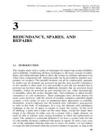
by a hierarchy diagram (H-diagram) such as that shown in Fig.
5
.
1
(a). The
diagram, which resembles an inverted tree, may be modeled as a mathe-
matical graph where each “box” in the diagram represents a node in the
graph and each line connecting the boxes represents a branch in the graph.
A node at level k (the predecessor) has several successor nodes at level
212
Associate
Cartesian position
with classification
Determine
Cartesian root

position
Find one root
through trial and
error
Solve function’s
quadratic equation
Use results to solve
for other roots
Check for validity
and requery if
incorrect
Query input file
Send data
to firm’s
plotting system
Interpret and
print results
Input (A, B, C, D)
Root Solution
Suspension
Design Program
Classify Roots
Plot Roots
0.0
1.0
2.0
3.0
4.0
1.1
1.2

2.1
2.2
2.3
3.1
3.2
4.1
4.2
0.0
1.0
2.0
3.0
4.0
1.1 1.2 2.1 2.2 2.3 3.1 3.2 4.1 4.2
H-DIAGRAM
(a)
(b)
Figure 5.1 (a), An H-diagram depicting the high-level architecture of a program to be used in designing the suspension system of a
high-speed train, assuming that the dynamics can be approximately modeled by a third-order system (characteristic polynomial is a
cubic); and (b), a graph corresponding to (a).
SOFTWARE DEVELOPMENT LIFE CYCLE
213
(k +
1
) (sometimes, the terms ancestor and descendant or parent and child
are used). The graph has no loops (cycles), all nodes are connected (you can
traverse a sequence of branches from any node to any other node), and the
graph is undirected (one can traverse all branches in either direction). Such a
graph is called a tree (free tree) and is shown in Fig.
5
.

1
(b). For more details
on trees, see Cormen [p.
91
ff.].
The example of the H-diagram given in Fig.
5
.
1
is for the top-level archi-
tecture of a program to be used in the hypothetical design of the suspension
system for a high-speed train. It is assumed that the dynamics of the suspen-
sion system can be approximated by a third-order differential equation and that
the stability of the suspension can be studied by plotting the variation in the
roots of the associated third-order characteristic polynomial (Ax
3
+ Bx
2
+ Cx
+ D

0
), which is a function of the various coefficients A, B, C, and D. It is
also assumed that the company already has a plotting program (
4
.
1
) that is to
be reused. The block (
4

.
2
) is to determine whether the roots have any positive
real parts, since this indicates instability. In a different design, one could move
the function
4
.
2
to
2
.
4
. Thus the H-diagram can be used to discuss differences
in high-level design architecture of a program. Of course, as one decomposes
a problem, modules may appear at different levels in the structure, so the H-
diagram need not be as symmetrical as that shown in Fig.
5
.
1
.
One feature of the top–down decomposition process is that the decision of
how to design lower-level elements is delayed until that level is reached in
the design decomposition and the final decision is delayed until coding of the
respective modules begins. This hiding process, called information hiding, is
beneficial, as it allows the designer to progress with his or her design while
more information is gathered and design alternatives are explored before a
commitment is made to a specific approach. If at each level k the project is
decomposed into very many subproblems, then that level becomes cluttered
with many concepts, at which point the tree becomes very wide. (The number
of successor nodes in a tree is called the degree of the predecessor node.) If the

decomposition only involves two or three subproblems (degree
2
or
3
), the tree
becomes very deep before all the modules are reached, which is again cum-
bersome. A suitable value to pick for each decomposition is
5
–
9
subprograms
(each node should have degree
5
–
9
). This is based on the work of the exper-
imental psychologist Miller [
1956
], who found that the classic human senses
(sight, smell, hearing, taste, and touch) could discriminate
5
–
9
logarithmic lev-
els. (See also Shooman [
1983
, pp.
194
,
195

].) Using the
5
–
9
decomposition
rule provides some bounds to the structure of the design process for an SPP.
Assume that the program size is N source lines of code (SLOC) in length.
If the graph is symmetrical and all the modules appear at the lowest level k,
as shown in Fig.
5
.
1
(a), and there are
5
–
9
successors at each node, then:
1
. All the levels above k represent program interfaces.
2
. At level
0
, there are between
5
0

1
and
9
0


1
interfaces. At level
1
, the
214
SOFTWARE RELIABILITY AND RECOVERY TECHNIQUES
top level node has between
5
1

5
and
9
1

9
interfaces. Also at level
2
are between
5
2

25
and
9
2

81
interfaces. Thus, for k levels starting

with level
0
, the sum of the geometric progression r
0
+ r
1
+ r
2
+·· ·+r
k
is
given by the equations that follow. (See Hall and Knight [
1957
, p.
39
]
or a similar handbook for more details.)
Sum

(r
k
−
1
)
/
(r −
1
)(
5
.

1
a)
and for r

5
to
9
, we have
(
5
k
−
1
)
/
4
≤ number of interfaces ≤ (
9
k
−
1
)
/
8
(
5
.
1
b)
3

. The number of modules at the lowest level is given by
5
k
≤ number of modules ≤
9
k
(
5
.
1
c)
4
. If each module is of size M, the number of lines of code is
M ×
5
k
≤ number of SLOC ≤ M ×
9
k
(
5
.
1
d)
Since modules generally vary in size, Eq. (
5
.
1
d) is still approximately correct
if M is replaced by the average value M.

We can better appreciate the use of Eqs. (
5
.
1
a–d) if we explore the following
example. Suppose that a module consists of
100
lines of code, in which case
M

100
, and it is estimated that a program design will take about
10
,
000
SLOC. Using Eq. (
5
.
1
c, d), we know that the number of modules must be
about
100
and that the number of levels are bounded by
5
k

100
and
9
k


100
. Taking logarithms and solving the resulting equations yields
2
.
09
≤ k ≤
2
.
86
. Thus, starting with the top-level
0
, we will have about
2
or
3
successor
levels. Similarly, we can bound the number of interfaces by Eq. (
5
.
1
b), and
substitution of k

3
yields the number of interfaces between
31
and
91
. Of

course, these computations are for a symmetric graph; however, they give us
a rough idea of the size of the H-diagram design and the number of modules
and interfaces that must be designed and tested.
5
.
3
.
6
Coding
Sometimes, a beginning undergraduate student feels that coding is the most
important part of developing software. Actually, it is only one of the six-
teen phases given in Table
5
.
1
. Previous studies [Shooman,
1983
, Table
5
.
1
]
have shown that coding constitutes perhaps
20
% of the total development
effort. The preceding phases of design—“start of project” through the “final
design”—entail about
40
% of the development effort; the remaining phases,
starting with the unit (module) test, are another

40
%. Thus coding is an impor-
tant part of the development process, but it does not represent a large fraction
of the cost of developing software. This is probably the first lesson that the
software engineering field teaches the beginning student.
SOFTWARE DEVELOPMENT LIFE CYCLE
215
The phases of software development that follow coding are various types of
testing. The design is an SPP, and the coding is assumed to follow the struc-
tured programming approach where the minimal basic control structures are
as follows: IF THEN ELSE and DO WHILE. In addition, most languages also
provide DO UNTIL, DO CASE, BREAK, and PROCEDURE CALL AND
RETURN structures that are often called extended control structures. Prior to
the
1970
s, the older, dangerous, and much-abused control structure GO TO
LABEL was often used indiscriminately and in a poorly thought-out manner.
One major thrust of structured programming was to outlaw the GO TO and
improve program structure. At the present, unless a programmer must correct,
modify, or adapt a very old (legacy) code, he or she should never or very sel-
dom encounter a GO TO. In a few specialized cases, however, an occasional
well-thought-out, carefully justified GO TO is warranted [Shooman,
1983
].
Almost all modern languages support structured programming. Thus the
choice of a language is based on other considerations, such as how familiar
the programmers are with the language, whether there is legacy code available,
how well the operating system supports the language, whether the code mod-
ules are to be written so that they may be reused in the future, and so forth.
Typical choices are C, Ada, and Visual Basic. In the case of OOP, the most

common languages at the present are C++ and Ada.
5
.
3
.
7
Testing
Testing is a complex process, and the exact nature of it depends on the design
philosophy and the phase of the project. If the design has progressed under a
top–down structured approach, it will be much like that outlined in Table
5
.
1
.
If the modern OOP techniques are employed, there may be more testing of
interfaces, objects, and other structures within the OOP philosophy. If proof of
program correctness is employed, there will be many additional layers added to
the design process involving the writing of proofs to ensure that the design will
satisfy a mathematical representation of the program logic. These additional
phases of design may replace some of the testing phases.
Assuming the top–down structured approach, the first step in testing the
code is to perform unit (module) testing. In general, the first module to be
written should be the main control structure of the program that contains the
highest interface levels. This main program structure is coded and tested first.
Since no additional code is generally present, sometimes “dummy” modules,
called test stubs, are used to test the interfaces. If legacy code modules are
available for use, clearly they can serve to test the interfaces. If a prototype
is to be constructed first, it is possible that the main control structure will be
designed well enough to be reused largely intact in the final version.
Each functional unit of code is subjected to a test, called unit or module

testing, to determine whether it works correctly by itself. For example, sup-
pose that company X pays an employee a base weekly salary determined by the
employee’s number of years of service, number of previous incentive awards,
216
SOFTWARE RELIABILITY AND RECOVERY TECHNIQUES
and number of hours worked in a week. The basic pay module in the payroll
program of the company would have as inputs the date of hire, the current
date, the number of hours worked in the previous week, and historical data
on the number of previous service awards, various deductions for withholding
tax, health insurance, and so on. The unit testing of this module would involve
formulating a number of hypothetical (or real) work records for a week plus a
number of hypothetical (or real) employees. The base pay would be computed
with pencil, paper, and calculator for these test cases. The data would serve
as inputs to the module, and the results (outputs) would be compared with the
precomputed results. Any discrepancies would be diagnosed, the internal cause
of the error (fault) would be located, and the code would be redesigned and
rewritten to correct the error. The tests would be repeated to verify that the error
had been eliminated. If the first code unit to be tested is the program control
structure, it would define the software interfaces to other modules. In addition,
it would allow the next phase of software testing—the integration test—to pro-
ceed as soon as a number of units had been coded and tested. During the inte-
gration test, one or more units of code would be added to the control structure
(and any previous units that had been integrated), and functional tests would be
performed along a path through the program involving the new unit(s) being
tested. Generally, only one unit would be integrated at a time to make localiz-
ing any errors easier, since they generally come from within the new module
of code; however, it is still possible for the error to be associated with the
other modules that had already completed the integration test. The integration
test would continue until all or most of the units have been integrated into the
maturing software system. Generally, module and many integration test cases

are constructed by examining the code. Such tests are often called white box
or clear box tests (the reason for these names will soon be explained).
The system test follows the integration test. During the system test, a sce-
nario is written encompassing an entire operational task that the software must
perform. For example, in the case of air traffic control software, one might
write a scenario that replicates aircraft arrivals and departures at Chicago’s
O’Hare Airport during a slow period—say, between
11
and
12
P
.
M
. This would
involve radar signals as inputs, the main computer and software for the sys-
tem, and one or more display processors. In some cases, the radar would not
be present, but simulated signals would be fed to the computer. (Anyone who
has seen the physical size of a large, modern radar can well appreciate why
the radar is not physically present, unless the system test is performed at an
air traffic control center, which is unlikely.) The display system is a “desk-
size” console likely to be present during the system test. As the system test
progresses, the software gradually approaches the time of release when it can
be placed into operation. Because most system tests are written based on the
requirements and specifications, they do not depend on the nature of the code;
they are as if the code were hidden from view in an opaque or black box.
Hence such functional tests are often called black box tests.
On large projects (and sometimes on smaller ones), the last phase of testing
SOFTWARE DEVELOPMENT LIFE CYCLE
217
is acceptance testing. This is generally written into the contract by the cus-

tomer. If the software is being written “in house,” an acceptance test would be
performed if the company software development procedures call for it. A typi-
cal acceptance test would contain a number of operational scenarios performed
by the software on the intended hardware, where the location would be chosen
from (a) the developer’s site, (b) the customer’s site, or (c) the site at which
the system is to be deployed. In the case of air traffic control (ATC), the ATC
center contains the present on-line system n and the previous system, n −
1
,as
a backup. If we call the new system n +
1
, it would be installed alongside n
and n −
1
and operate on the same data as the on-line system. Comparing the
outputs of system n+
1
with system n for a number of months would constitute
a very good acceptance test. Generally, the criterion for acceptance is that the
software must operate on real or simulated system data for a specified number
of hours or be subjected to a certain number of test inputs. If the acceptance
test is passed, the software is accepted and the developer is paid; however, if
the test is failed, the developer resumes the testing and correcting of software
errors (including those found during the acceptance test), and a new acceptance
test date is scheduled.
Sometimes, “third party” testing is used, in which the customer hires an out-
side organization to make up and administer integration, system, or acceptance
tests. The theory is that the developer is too close to his or her own work and
cannot test and evaluate it in an unbiased manner. The third party test group
is sometimes an independent organization within the developer’s company. Of

course, one wonders how independent such an in-house group can be if it and
the developers both work for the same boss.
The term regression testing is often used, describing the need to retest the
software with the previous test cases after each new error is corrected. In the-
ory, one must repeat all the tests; however, a selected subset is generally used
in the retest. Each project requires a test plan to be written early in the develop-
ment cycle in parallel with or immediately following the completion of speci-
fications. The test plan documents the tests to be performed, organizes the test
cases by phase, and contains the expected outputs for the test cases. Generally,
testing costs and schedules are also included.
When a commercial software company is developing a product for sale to
the general business and home community, the later phases of testing are often
somewhat different, for which the terms alpha testing and beta testing are often
used. Alpha testing means that a test group within the company evaluates the
software before release, whereas beta testing means that a number of “selected
customers” with whom the developer works are given early releases of the
software to help test and debug it. Some people feel that beta testing is just a
way of reducing the cost of software development and that it is not a thorough
way of testing the software, whereas others feel that the company still does
adequate testing and that this is just a way of getting a lot of extra field testing
done in a short period of time at little additional cost.
During early field deployment, additional errors are found, since the actual
218
SOFTWARE RELIABILITY AND RECOVERY TECHNIQUES
operating environment has features or inputs that cannot be simulated. Gener-
ally, the developer is responsible for fixing the errors during early field deploy-
ment. This responsibility is an incentive for the developer to do a thorough
job of testing before the software is released because fixing errors after it is
released could cost
25

–
100
times as much as that during the unit test. Because
of the high cost of such testing, the contract often includes a warranty period
(of perhaps
1
–
2
years or longer) during which the developer agrees to fix any
errors for a fee.
If the software is successful, after a period of years the developer and others
will probably be asked to provide a proposal and estimate the cost of including
additional features in the software. The winner of the competition receives a
new contract for the added features. If during initial development the devel-
oper can determine something about possible future additions, the design can
include the means of easily implementing these features in the future, a process
for which the term “putting hooks” into the software is often used. Eventually,
once no further added features are feasible or if the customer’s needs change
significantly, the software is discarded.
5
.
3
.
8
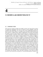
Diagrams Depicting the Development Process
The preceding discussion assumed that the various phases of software develop-
ment proceed in a sequential fashion. Such a sequence is often called waterfall
development because of the appearance of the symbolic model as shown in
Fig.
5

.
2
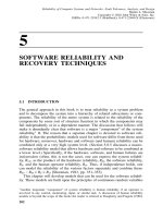
. This figure does not include a prototype phase; if this is added to the
development cycle, the diagram shown in Fig.
5
.
3
ensues. In actual practice,
portions of the system are sometimes developed and tested before the remain-
ing portions. The term software build is used to describe this process; thus
one speaks of build
4
being completed and integrated into the existing system
composed of builds
1
–
3
. A diagram describing this build process, called the
incremental model of software development, is given in Fig.
5
.
4
. Other related
models of software development are given in Schach [
1999
].
Now that the general features of the development process have been
described, we are ready to introduce software reliability models related to the
software development process.
5

.
4
RELIABILITY THEORY
5
.
4
.
1
Introduction
In Section
5
.
1
, software reliability was defined as the probability that the soft-
ware will perform its intended function, that is, the probability of success,
which is also known as the reliability. Since we will be using the principles
of reliability developed in Appendix B, Section B
3
, we summarize the devel-
opment of reliability theory that is used as a basis for our software reliability
models.
RELIABILITY THEORY
219
Requirements
Phase
Changed
Requirements
Specification
Phase
Design

Phase
Implementation
Phase
Integration
Phase
Operations
Mode
Retirement
Verify Verify
Verify
Verify
Test
Test
SOFTWARE LIFE-CYCLE
DEVELOPMENT MODELS
(WATERFALL MODEL)
Development
Maintenance
Figure
5
.
2
Diagram of the waterfall model of software development.
5
.
4
.
2
Reliability as a Probability of Success
The reliability of a system (hardware, software, human, or a combination

thereof) is the probability of success, P
s
, which is unity minus the probability
of failure, P
f
. If we assume that t is the time of operation, that the operation
starts at t

0
, and that the time to failure is given by t
f
, we can then express
the reliability as
R(t)

P
s

P(t
f
≥ t)

1
− P
f

1
− P(
0
≤ t

f
≤ t)(
5
.
2
)
220
SOFTWARE RELIABILITY AND RECOVERY TECHNIQUES
Rapid
Prototype
Changed
Requirements
Specification
Phase
Design
Phase
Implementation
Phase
Integration
Phase
Operations
Mode
Retirement
Verify Verify
Verify
Verify
Test
Test
SOFTWARE LIFE-CYCLE
DEVELOPMENT MODELS

(RAPID PROTOTYPE MODEL)
Development
Maintenance
Figure
5
.
3
Diagram of the rapid prototype model of software development.
The notation, P(
0
≤ t
f
≤ t), in Eq. (
5
.
2
) stands for the probability that the time
to failure is less than or equal to t. Of course, time is always a positive value,
so the time to failure is always equal to or greater than
0
. Reliability can also
be expressed in terms of the cumulative probability distribution function for
the random variable time to failure, F(t), and the probability density function,
f (t) (see Appendix A, Section A
6
). The density function is the derivative of
the distribution function, f (t)

dF(t)
/

dt, and the distribution function is the
RELIABILITY THEORY
221
Requirements
Phase
Specification
Phase
Architectural
Design
Verify
Verify
Verify
Operations Mode
Retirement
SOFTWARE LIFE-CYCLE
DEVELOPMENT MODELS
(INCREMENTAL MODEL WITH BUILDS)
Development
Maintenance
For each build, perform
a detailed design,
implementation, and
integration. Test; then
deliver to client.
Figure
5
.
4
Diagram of the incremental model of software development.
integral of the density function, F(t)


1
−
∫
f (t) dt. Since by definition F(t)

P(
0
≤ t
f
≤ t), Eq. (
5
.
2
) becomes
R(t)

1
− F(t)

1
−
∫
f (t) dt (
5
.
3
)
Thus reliability can be easily calculated if the probability density function for
the time to failure is known. Equation (

5
.
3
) states the simple relationships
among R(t), F(t), and f (t); given any one of the functions, the other two are
easy to calculate.
222
SOFTWARE RELIABILITY AND RECOVERY TECHNIQUES
5
.
4
.
3
Failure-Rate (Hazard) Function
Equation (
5
.
3
) expresses reliability in terms of the traditional mathematical
probability functions, F(t), and f (t); however, reliability engineers have found
these functions to be generally ill-suited for study if we want intuition, fail-
ure data interpretation, and mathematics to agree. Intuition suggests that we
study another function—a conditional probability function called the failure
rate (hazard), z(t). The following analysis develops an expression for the reli-
ability in terms of z(t) and relates z(t) to f (t) and F(t).
The probability density function can be interpreted from the following rela-
tionship:
P(t < t
f
< t + dt)


P(failure in interval t to t + dt)

f (t) dt (
5
.
4
)
One can relate the probability functions to failure data analysis if we begin with
N items placed on the life test at time t. The number of items surviving the
life test up to time t is denoted by n(t). At any point in time, the probability of
failure in interval dt is given by (number of failures)
/
N. (To be mathematically
correct, we should say that this is only true in the limit as dt 
0
.) Similarly,
the reliability can be expressed as R(t)

n(t)
/
N. The number of failures in
interval dt is given by [n(t) − n(t + dt)], and substitution in Eq. (
5
.
4
) yields
n(t) − n(t + dt)
N


f (t) dt (
5
.
5
)
However, we can also write Eq. (
5
.
4
) as
f (t) dt

P(no failure in interval
0
to t)
× P(failure in interval dt
|
no failure in interval
0
to t)(
5
.
6
a)
The last expression in Eq. (
5
.
6
a) is a conditional failure probability, and the
symbol

|
is interpreted as “given that.” Thus P(failure in interval dt
|
no failure
in interval
0
to t) is the probability of failure in
0
to t given that there was no
failure up to t, that is, the item is working at time t. By definition, P(failure
in interval dt
|
no failure in interval
0
to t) is called the hazard function, z(t);
its more popular name is the failure-rate function. Since the probability of no
failure is just the reliability function, Eq. (
5
.
6
a) can be written as
f (t) dt

R(t) × z(t) dt (
5
.
6
b)
This equation relates f (t), R(t), and z(t); however, we will develop a more
convenient relationship shortly.

Substitution of Eq. (
5
.
6
b) into Eq. (
5
.
5
) along with the relationship R(t)

n(t)
/
N yields
RELIABILITY THEORY
223
n(t) − n(t + dt)
N

R(t)z(t) dt

n(t)
N
z(t) dt (
5
.
7
)
Solving Eqs. (
5
.

5
) and (
5
.
7
) for f (t) and z(t), we obtain
f (t)

n(t) − n(t + dt)
N dt
(
5
.
8
)
z(t)

n(t) − n(t + dt)
n(t) dt
(
5
.
9
)
Comparing Eqs. (
5
.
8
) and (
5

.
9
), we see that f (t) reflects the rate of failure
based on the original number N placed on test, whereas z(t) gives the instan-
taneous rate of failure based on the number of survivors at the beginning of
the interval.
We can develop an equation for R(t) in terms of z(t) from Eq. (
5
.
6
b):
z(t)

f (t)
R(t)
(
5
.
10
)
and from Eq. (
5
.
3
), differentiation of both sides yields
dR(t)
dt

−f (t)(
5

.
11
)
Substituting Eq. (
5
.
11
) into (
5
.
10
) and solving for z(t) yields
z(t)

−
dR(t)
dt
΋
R(t)(
5
.
12
)
This differential equation can be solved by integrating both sides, yielding
ln{R(t)}

−
∫
z(t) dt (
5

.
13
a)
Eliminating the natural logarithmic function in this equation by exponentiating
both sides yields
R(t)

e
−
∫
z(t) dt
(
5
.
13
b)
which is the form of the reliability function that is used in the following model
development.
If one substitutes limits for the integral, a dummy variable, x, is required
inside the integral, and a constant of integration must be added, yielding
224
SOFTWARE RELIABILITY AND RECOVERY TECHNIQUES
R(t)

e
−
∫
t
0
z(x) dx+ A


Be
−
∫
t
0
z(x) dx
(
5
.
13
c)
As is normally the case in the solution of differential equations, the constant
B

e
−A
is evaluated from the initial conditions. At t

0
, the item is good and
R(t

0
)

1
. The integral from
0
to

0
is
0
; thus B

1
and Eq. (
5
.
13
c) becomes
R(t)

e
−
∫
t
0
z(x) dx
(
5
.
13
d)
5
.
4
.
4
Mean Time To Failure

Sometimes, the complete information on failure behavior, z(t) or f (t), is not
needed, and the reliability can be represented by the mean time to failure
(MTTF) rather than the more detailed reliability function. A point estimate
(MTTF) is given instead of the complete time function, R(t). A rough analogy
is to rank the strength of a hitter in baseball in terms of his or her batting aver-
age, rather than the complete statistics of how many times at bat, how many
first-base hits, how many second-base hits, and so on.
The mean value of a probability function is given by the expected value,
E(t), of the random variable, which is given by the integral of the product of
the random variable (time to failure) and its density function, which has the
following form:
MTTF

E(t)

∫
∞
0
tf(t) dt (
5
.
14
)
Some mathematical manipulation of Eq. (
5
.
14
) involving integration by parts
[Shooman,
1990

] yields a simpler expression:
MTTF

E(t)

∫
∞
0
R(t) dt (
5
.
15
)
Sometimes, the mean time to failure is called mean time between failure
(MTBF), and although there is a minor difference in their definitions, we will
use the terms interchangeably.
5
.
4
.
5
Constant-Failure Rate
In general, a choice of the failure-rate function defines the reliability model.
Such a choice should be made based on past studies that include failure-rate
data or reasonable engineering assumptions. In several practical cases, the fail-
ure rate is constant in time, z(t)

l, and the mathematics becomes quite simple.
Substitution into Eqs. (
5

.
13
d) and (
5
.
15
) yields
SOFTWARE ERROR MODELS
225
R(t)

e
−
∫
t
0
l dx

e
−lt
(
5
.
16
)
MTTF

E(t)

∫

∞
0
e
−lt
dt

1
l
(
5
.
17
)
The result is particularly simple: the reliability function is a decreasing expo-
nential function where the exponent is the negative of the failure rate l. A
smaller failure rate means a slower exponential decay. Similarly, the MTTF is
just the reciprocal of the failure rate, and a small failure rate means a large
MTTF.
As an example, suppose that past life tests have shown that an item fails at
a constant-failure rate. If
100
items are tested for
1
,
000
hours and
4
of these
fail, then l


4
/
(
100
×
1
,
000
)

4
×
10
−
5
. Substitution into Eq. (
5
.
17
) yields
MTTF

25
,
000
hours. Suppose we want the reliability for
5
,
000
hours; in that

case, substitution into Eq. (
5
.
16
) yields R(
5
,
000
)

e
−(
4
/
100
,
000
) ×
5
,
000

e
−
0
.
2

0
.

82
. Thus, if the failure rate were constant at
4
×
10
−
5
, the MTTF is
25
,
000
hours, and the reliability (probability of no failures) for
5
,
000
hours is
0
.
82
.
More complex failure rates yield more complex results. If the failure rate
increases with time, as is often the case in mechanical components that even-
tually “wear out,” the hazard function could be modeled by z(t)

kt. The
reliability and MTTF then become the equations that follow [Shooman,
1990
].
R(t)


e
−
∫
t
0
kxdx

e
−kt
2
/
2
(
5
.
18
)
MTTF

E(t)

∫
∞
0
e
−kt
2
/
2
dt



p
2
k
(
5
.
19
)
Other choices of hazard functions would give other results.
The reliability mathematics of this section applies to hardware failure and
human errors, and also to software errors if we can characterize the software
errors by a failure-rate function. The next section discusses how one can for-
mulate a failure-rate function for software based on a software error model.
5
.
5
SOFTWARE ERROR MODELS
5
.
5
.
1
Introduction
Many reliability models discussed in the remainder of this chapter are related
to the number of residual errors in the software; therefore, this section dis-
cusses software error models. Generally, one speaks of faults in the code that
cause errors in the software operation; it is these errors that lead to system
failure. Software engineers differentiate between a fault, a software error, and

a software-caused system failure only when necessary, and the slang expres-
226
SOFTWARE RELIABILITY AND RECOVERY TECHNIQUES
sion “software bug” is commonly used in normal conversation to describe a
software problem.
3
Software errors occur at many stages in the software life cycle. Errors may
occur in the requirements-and-specifications phase. For example, the specifi-
cations might state that the time inputs to the system from a precise cesium
atomic clock are in hours, minutes, and seconds when actually the clock out-
put is in hours and decimal fractions of an hour. Such an erroneous specifica-
tion might be found early in the development cycle, especially if a hardware
designer familiar with the cesium clock is included in the specification review.
It is also possible that such an error will not be found until a system test, when
the clock output is connected to the system. Errors in requirements and speci-
fications are identified as separate entities; however, they will be added to the
code faults in this chapter. If the range safety officer has to destroy a satellite
booster because it is veering off course, it matters little to him or her whether
the problem lies in the specifiations or whether it is a coding error.
Errors occur in the program logic. For example, the THEN and ELSE
clauses in an IF THEN ELSE statement may be interchanged, creating an error,
or a loop is erroneously executed n−
1
times rather than the correct value, which
is n times. When a program is coded, syntax errors are always present and are
caught by the compiler. Such syntax errors are too frequent, embarrassing, and
universal to be considered errors.
Actually, design errors should be recorded once the program management
reviews and endorses a preliminary design expressed by a set of design repre-
sentations (H-diagrams, control graphs, and maybe other graphical or abbrevi-

ated high-level control-structure code outlines called pseudocodes) in addition
to requirements and specifications. Often, a formal record of such changes is
not kept. Furthermore, errors found by code reading and testing at the middle
(unit) code level (called module errors) are often not carefully kept. A change
in the preliminary design and the occurrence of module test errors should both
be carefully recorded.
Oftentimes, the standard practice is not to start counting software errors,
3
The origin of the word “bug” is very interesting. In the early days of computers, many of the
machines were constructed of vacuum tubes and relays, used punched cards for input, and used
machine language or assembly language. Grace Hopper, one of the pioneers who developed
the language COBOL and who spent most of her career in the U.S. Navy (rising to the rank
of admiral), is generally credited with the expression. One hot day in the summer of
1945
at
Harvard, she was working on the Mark II computer (successor to the pioneering Mark I) when
the machine stopped. Because there was no air conditioning, the windows were opened, which
permitted the entry of a large moth that (subsequent investigation revealed) became stuck between
the contacts of one of the relays, thereby preventing the machine from functioning. Hopper and
the team removed the moth with tweezers; later, it was mounted in a logbook with tape (it is now
displayed in the Naval Museum at the Naval Surface Weapons Center in Dahlgren, Virginia).
The expression “bug in the system” soon became popular, as did the term “debugging” to denote
the fixing of program errors. It is probable that “bug” was used before this incident during World
War II to describe system or hardware problems, but this incident is clearly the origin of the term
“software bug” [Billings,
1989
, p.
58
].