Độ tin cậy của hệ thống máy tính và mạng P2

2
CODING TECHNIQUES
Reliability of Computer Systems and Networks: Fault Tolerance, Analysis, and Design
Martin L. Shooman
Copyright 
2002
John Wiley & Sons, Inc.
ISBNs:
0
-
471
-
29342
-
3
(Hardback);
0
-
471
-
22460
-X (Electronic)
30
2
.
1
INTRODUCTION
Many errors in a computer system are committed at the bit or byte level when
information is either transmitted along communication lines from one computer
to another or else within a computer from the memory to the microprocessor
or from microprocessor to input

/
output device. Such transfers are generally
made over high-speed internal buses or sometimes over networks. The simplest
technique to protect against such errors is the use of error-detecting and error-
correcting codes. These codes are discussed in this chapter in this context. In
Section
3
.
9
, we see that error-correcting codes are also used in some versions
of RAID memory storage devices.
The reader should be familiar with the material in Appendix A and Sections
B
1
–B
4
before studying the material of this chapter. It is suggested that this
material be reviewed briefly or studied along with this chapter, depending on
the reader’s background.
The word code has many meanings. Messages are commonly coded and
decoded to provide secret communication [Clark,
1977
; Kahn,
1967
], a prac-
tice that technically is known as cryptography. The municipal rules governing
the construction of buildings are called building codes. Computer scientists
refer to individual programs and collections of programs as software, but many
physicists and engineers refer to them as computer codes. When information
in one system (numbers, alphabet, etc.) is represented by another system, we

call that other system a code for the first. Examples are the use of binary num-
bers to represent numbers or the use of the ASCII code to represent the letters,
numerals, punctuation, and various control keys on a computer keyboard (see
INTRODUCTION
31
Table C.
1
in Appendix C for more information). The types of codes that we
discuss in this chapter are error-detecting and -correcting codes. The principle
that underlies error-detecting and -correcting codes is the addition of specially
computed redundant bits to a transmitted message along with added checks
on the bits of the received message. These procedures allow the detection and
sometimes the correction of a modest number of errors that occur during trans-
mission.
The computation associated with generating the redundant bits is called cod-
ing; that associated with detection or correction is called decoding. The use
of the words message, transmitted, and received in the preceding paragraph
reveals the origins of error codes. They were developed along with the math-
ematical theory of information largely from the work of C. Shannon [
1948
],
who mentioned the codes developed by Hamming [
1950
] in his original article.
(For a summary of the theory of information and the work of the early pio-
neers in coding theory, see J. R. Pierce [
1980
, pp.
159
–

163
].) The preceding
use of the term transmitted bits implies that coding theory is to be applied to
digital signal transmission (or a digital model of analog signal transmission), in
which the signals are generally pulse trains representing various sequences of
0
s and
1
s. Thus these theories seem to apply to the field of communications;
however, they also describe information transmission in a computer system.
Clearly they apply to the signals that link computers connected by modems
and telephone lines or local area networks (LANs) composed of transceivers,
as well as coaxial wire and fiber-optic cables or wide area networks (WANs)
linking computers in distant cities. A standard model of computer architecture
views the central processing unit (CPU), the address and memory buses, the
input
/
output (I
/
O) devices, and the memory devices (integrated circuit memory
chips, disks, and tapes) as digital signal (computer word) transmission, stor-
age, manipulation, generation, and display devices. From this perspective, it is
easy to see how error-detecting and -correcting codes are used in the design of
modems, memory stems, disk controllers (optical, hard, or floppy), keyboards,
and printers.
The difference between error detection and error correction is based on the
use of redundant information. It can be illustrated by the following electronic
mail message:
Meet me in Manhattan at the information desk at Senn Station on July
43

. I will
arrive at
12
noon on the train from Philadelphia.
Clearly we can detect an error in the date, for extra information about the cal-
endar tells us that there is no date of July
43
. Most likely the digit should be a
1
or a
2
, but we can’t tell; thus the error can’t be corrected without further infor-
mation. However, just a bit of extra knowledge about New York City railroad
stations tells us that trains from Philadelphia arrive at Penn (Pennsylvania) Sta-
tion in New York City, not the Grand Central Terminal or the PATH Terminal.
Thus, Senn is not only detected as an error, but is also corrected to Penn. Note
32
CODING TECHNIQUES
that in all cases, error detection and correction required additional (redundant)
information. We discuss both error-detecting and error-correcting codes in the
sections that follow. We could of course send return mail to request a retrans-
mission of the e-mail message (again, redundant information is obtained) to
resolve the obvious transmission or typing errors.
In the preceding paragraph we discussed retransmission as a means of cor-
recting errors in an e-mail message. The errors were detected by a redundant
source and our knowledge of calendars and New York City railroad stations. In
general, with pulse trains we have no knowledge of “the right answer.” Thus if
we use the simple brute force redundancy technique of transmitting each pulse
sequence twice, we can compare them to detect errors. (For the moment, we
are ignoring the rare situation in which both messages are identically corrupted

and have the same wrong sequence.) We can, of course, transmit three times,
compare to detect errors, and select the pair of identical messages to provide
error correction, but we are again ignoring the possibility of identical errors
during two transmissions. These brute force methods are inefficient, as they
require many redundant bits. In this chapter, we show that in some cases the
addition of a single redundant bit will greatly improve error-detection capabili-
ties. Also, the efficient technique for obtaining error correction by adding more
than one redundant bit are discussed. The method based on triple or N copies
of a message are covered in Chapter
4
. The coding schemes discussed so far
rely on short “noise pulses,” which generally corrupt only one transmitted bit.
This is generally a good assumption for computer memory and address buses
and transmission lines; however, disk memories often have sequences of errors
that extend over several bits, or burst errors, and different coding schemes are
required.
The measure of performance we use in the case of an error-detecting code
is the probability of an undetected error, P
ue
, which we of course wish to min-
imize. In the case of an error-correcting code, we use the probability of trans-
mitted error, P
e
, as a measure of performance, or the reliability, R, (probability
of success), which is (
1
− P
e
). Of course, many of the more sophisticated cod-
ing techniques are now feasible because advanced integrated circuits (logic and

memory) have made the costs of implementation (dollars, volume, weight, and
power) modest.
The type of code used in the design of digital devices or systems largely
depends on the types of errors that occur, the amount of redundancy that is cost-
effective, and the ease of building coding and decoding circuitry. The source
of errors in computer systems can be traced to a number of causes, including
the following:
1
. Component failure
2
. Damage to equipment
3
. “Cross-talk” on wires
4
. Lightning disturbances
INTRODUCTION
33
5
. Power disturbances
6
. Radiation effects
7
. Electromagnetic fields
8
. Various kinds of electrical noise
Note that we can roughly classify sources
1
,
2
, and

3
as causes that are internal
to the equipment; sources
4
,
6
, and
7
as generally external causes; and sources
5
and
6
as either internal or external. Classifying the source of the disturbance is
only useful in minimizing its strength, decreasing its frequency of occurrence,
or changing its other characteristics to make it less disturbing to the equipment.
The focus of this text is what to do to protect against these effects and how the
effects can compromise performance and operation, assuming that they have
occurred. The reader may comment that many of these error sources are rather
rare; however, our desire for ultrareliable, long-life systems makes it important
to consider even rare phenomena.
The various types of interference that one can experience in practice can
be illustrated by the following two examples taken from the aircraft field.
Modern aircraft are crammed full of digital and analog electronic equipment
that are generally referred to as avionics. Several recent instances of military
crashes and civilian troubles have been noted in modern electronically con-
trolled aircraft. These are believed to be caused by various forms of electro-
magnetic interference, such as passenger devices (e.g., cellular telephones);
“cross-talk” between various onboard systems; external signals (e.g., Voice
of America Transmitters and Military Radar); lightning; and equipment mal-
function [Shooman,

1993
]. The systems affected include the following: auto-
pilot, engine controls, communication, navigation, and various instrumentation.
Also, a previous study by Cockpit (the pilot association of Germany) [Taylor,
1988
, pp.
285
–
287
] concluded that the number of soft fails (probably from
alpha particles and cosmic rays affecting memory chips) increased in modern
aircraft. See Table
2
.
1
for additional information.
TABLE
2
.
1
Increase of Soft Fails with Airplane Generation
Altitude (
1
,
000
s feet) Soft
Airplane Total No. of Fails
Type Ground-
55
–

20 20
–
3030
+ Reports Aircraft per a
/
c
B
707 2 0 0 2 4 14 0
.
29
B
727
/
737 11 7 2 4 24 39
/
28 0
.
36
B
747 11 0 1 6 18 10 1
.
80
DC
10 21 5 0 29 55 134
.
23
A
300 96 12 6 17 131 10 13
.
10

Source: [Taylor,
1988
].
34
CODING TECHNIQUES
It is not clear how the number of flight hours varied among the different
airplane types, what the computer memory sizes were for each of the aircraft,
and the severity level of the fails. It would be interesting to compare this data
to that observed in the operation of the most advanced versions of B
747
and
A
320
aircraft, as well as other more recent designs.
There has been much work done on coding theory since
1950
[Rao,
1989
].
This chapter presents a modest sampling of theory as it applies to fault-tolerant
systems.
2
.
2
BASIC PRINCIPLES
Coding theory can be developed in terms of the mathematical structure of
groups, subgroups, rings, fields, vector spaces, subspaces, polynomial algebra,
and Galois fields [Rao,
1989
, Chapter

2
]. Another simple yet effective devel-
opment of the theory based on algebra and logic is used in this text [Arazi,
1988
].
2
.
2
.
1
Code Distance
We will deal with strings of binary digits (
0
or
1
), which are of specified length
and called the following synonymous terms: binary block, binary vector, binary
word, or just code word. Suppose that we are dealing with a
3
-bit message (b
1
,
b
2
, b
3
) represented by the bits x
1
, x
2

, x
3
. We can speak of the eight combi-
nations of these bits—see Table
2
.
2
(a)—as the code words. In this case they
are assigned according to the sequence of binary numbers. The distance of a
code is the minimum number of bits by which any one code word differs from
another. For example, the first and second code words in Table
2
.
2
(a) differ
only in the right-most digit and have a distance of
1
, whereas the first and the
last code words differ in all
3
digits and have a distance of
3
. The total number
of comparisons needed to check all of the word pairs for the minimum code
distance is the number of combinations of
8
items taken
2
at a time
΂

8
2
΃
, which
is equal to
8
!
/
2
!
6
!

28
.
A simpler way of visualizing the distance is to use the “cube method” of
displaying switching functions. A cube is drawn in three-dimensional space (x,
y, z), and a main diagonal goes from x

y

z

0
to x

y

z


1
. The distance
is the number of cube edges between any two code words that represent the
vertices of the cube. Thus, the distance between
000
and
001
is a single cube
edge, but the distance between
000
and
111
is
3
since
3
edges must be traversed
to get between the two vertices. (In honor of one of the pioneers of coding
theory, the code distance is generally called the Hamming distance.) Suppose
that noise changes a single bit of a code word from
0
to
1
or
1
to
0
. The
first code word in Table
2

.
2
(a) would be changed to the second, third, or fifth,
depending on which bit was corrupted. Thus there is no way to detect a single-
bit error (or a multibit error), since any change in a code word transforms it
BASIC PRINCIPLES
35
TABLE
2
.
2
Examples of
3
- and
4
-Bit Code Words
(b)
4
-Bit Code Words: (c)
(a)
3
Original Bits plus Illegal Code Words
3
-Bit Code Added Even-Parity for the Even-Parity
Words (Legal Code Words)
Code of (b)
x
1
x
2

x
3
x
1
x
2
x
3
x
4
x
1
x
2
x
3
x
4
b
1
b
2
b
3
p
1
b
1
b
2

b
3
p
1
b
1
b
2
b
3
00 0 0 0 0 0 1 0 0 0
00 1 1 0 0 1 0 0 0 1
01 0 1 0 1 0 0 0 1 0
01 1 0 0 1 1 1 0 1 1
10 0 1 1 0 0 0 1 0 0
10 1 0 1 0 1 1 1 0 1
11 0 0 1 1 0 1 1 1 0
11 1 1 1 1 1 0 1 1
1
into another legal code word. One can create error-detecting ability in a code
by adding check bits, also called parity bits, to a code.
The simplest coding scheme is to add one redundant bit. In Table
2
.
2
(b), a
single check bit (parity bit p
1
) is added to the
3

-bit code words b
1
, b
2
, and b
3
of Table
2
.
2
(a), creating the eight new code words shown. The scheme used
to assign values to the parity bit is the coding rule; in this case, p
1
is chosen
so that the number of one bits in each word is an even number. Such a code is
called an even-parity code, and the words in Table
2
.
1
(b) become legal code
words and those in Table
2
.
1
(c) become illegal code words. Clearly we could
have made the number of one bits in each word an odd number, resulting in
an odd-parity code, and so the words in Table
2
.
1

(c) would become the legal
ones and those in
2
.
1
(b) become illegal.
2
.
2
.
2
Check-Bit Generation and Error Detection
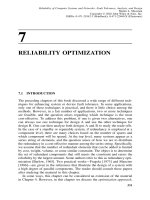
The code generation rule (even parity) used to generate the parity bit in Table
2
.
2
(b) will now be used to design a parity-bit generator circuit. We begin with
a Karnaugh map for the switching function p
1
(b
1
, b
2
, and b
3
) where the parity
bit is a function of the three code bits as given in Fig.
2
.
1

(a). The resulting
Karnaugh map is given in this figure. The top left cell in the map corresponds
to p
1

0
when b
1
, b
2
, and b
3

000
, whereas the top right cell represents p
1

1
when b
1
, b
2
, and b
3

001
. These two cells represent the first two rows
of Table
2
.

2
(b); the other cells in the map represent the other six rows in the
table. Since none of the ones in the Karnaugh map touch, no simplification is
possible, and there are four minterms in the circuit, each generated by the four
gates shown in the circuit. The OR gate “collects” these minterms, generating
a parity check bit p
1
whenever a sequence of pulses b
1
, b
2
, and b
3
occurs.
36
CODING TECHNIQUES
b′
1
b′
1
b
1
b
1
b′
2
b
2
b
2

b′
2
b
3
b′
3
b
3
b′
3
Parity
Bit
Circuit for
Parity-Bit Generation
01
00 01
01
01
11
10
10
10
b
3
b
12
b
Karnaugh Map for
Parity-Bit Generation
p

1
′
p
1
′
p
1
′
p
1
′
p
1
p
1
b
1
b
1
′
b
1
b
1
b
1
b
1
′
b

2
′
b
2
b
2
′
b
2
b
2
′
b
2
b
3
b
3
′
b
3
′
b
3
b
3
p
1
b
1

′
b
2
′
b
3
′
p
1
b
1
b
2
b
3
′
b
3
Error
Detection
Circuit for
Error Detection
00 1101 10
00 1100
1100
01
11
10
0011
0011

p
11
b
b
23
b
Karnaugh Map for
Error Detection
(a)
(b)
Figure
2
.
1
Elementary parity-bit coding and decoding circuits. (a) Generation of an
even-parity bit for a
3
-bit code word. (b) Detection of an error for an even-parity-bit
code for a
3
-bit code word.
PARITY-BIT CODES
37
The addition of the parity bit creates a set of legal and illegal words; thus
we can detect an error if we check for legal or illegal words. In Fig.
2
.
1
(b) the
Karnaugh map displays ones for legal code words and zeroes for illegal code

words. Again, there is no simplification since all the minterms are separated,
so the error detector circuit can be composed by generating all the illegal word
minterms (indicated by zeroes) in Fig.
2
.
1
(b) using eight AND gates followed
by an
8
-input OR gate as shown in the figure. The circuits derived in Fig.
2
.
1
can be simplified by using exclusive or (EXOR) gates (as shown in the
next section); however, we have demonstrated in Fig.
2
.
1
how check bits can
be generated and how errors can be detected. Note that parity checking will
detect errors that occur in either the message bits or the parity bit.
2
.
3
PARITY-BIT CODES
2
.
3
.
1

Applications
Three important applications of parity-bit error-checking codes are as follows:
1
. The transmission of characters over telephone lines (or optical, micro-
wave, radio, or satellite links). The best known application is the use of
a modem to allow computers to communicate over telephone lines.
2
. The transmission of data to and from electronic memory (memory read
and write operations).
3
. The exchange of data between units within a computer via various data
and control buses.
Specific implementation details may differ among these three applications, but
the basic concepts and circuitry are very similar. We will discuss the first appli-
cation and use it as an illustration of the basic concepts.
2
.
3
.
2
Use of Exclusive OR Gates
This section will discuss how an additional bit can be added to a byte for error
detection. It is common to represent alphanumeric characters in the input and
output phases of computation by a single byte. The ASCII code is almost uni-
versally used. One technique uses the entire byte to represent
2
8

256
possible

characters (the extended character set that is used on IBM personal computers,
containing some Greek letters, language accent marks, graphic characters, and
so forth, as well as an additional ninth parity bit. The other approach limits
the character set to
128
, which can be expressed by seven bits, and uses the
eighth bit for parity.
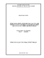
Suppose we wish to build a parity-bit generator and code checker for the
case of seven message bits and one parity bit. Identifying the minterms will
reveal a generalization of the checkerboard diagram similar to that given in the
38
CODING TECHNIQUES
p
1
b
1
b
2
b
3
b
4
b
5
b
6
b
7
Parity bit
Message bits

Control
signal
1 = odd parity
0 = even parity
Inputs
Output-
g
enerated
parity bit
pbbbbbbb
1
=
1234567
⊕⊕⊕⊕⊕⊕
Inputs
Outputs
p
1
b
1
b
2
b
3
b
4
b
5
b
6

b
7
even parity odd parity
1 = error
0 = OK
1 = error
0 = OK
(a) Parity-Bit Encoder (generator)
(b) Parity-Bit Decoder (checker)
Figure
2
.
2
Parity-bit encoder and decoder for a transmitted byte: (a) A
7
-bit parity
encoder ( generator); (b) an
8
-bit parity decoder (checker).
Karnaugh maps of Fig.
2
.
1
. Such checkerboard patterns indicate that EXOR
gates can be used to simplify the circuit. A circuit using EXOR gates for parity-
bit generation and for checking of an
8
-bit byte is given in Fig.
2
.

2
. Note that
the circuit in Fig.
2
.
2
(a) contains a control input that allows one to easily switch
from even to odd parity. Similarly, the addition of the NOT gate (inverter) at
the output of the checking circuit allows one to use either even or odd parity.
PARITY-BIT CODES
39
Most modems have these refinements, and a switch chooses either even or odd
parity.
2
.
3
.
3
Reduction in Undetected Errors
The purpose of parity-bit checking is to detect errors. The extent to which
such errors are detected is a measure of the success of the code, whereas the
probability of not detecting an error, P
ue
, is a measure of failure. In this section
we analyze how parity-bit coding decreases P
ue
. We include in this analysis
the reliability of the parity-bit coding and decoding circuit by analyzing the
reliability of a standard IC parity code generator
/

checker. We model the failure
of the IC chip in a simple manner by assuming that it fails to detect errors, and
we ignore the possibility that errors are detected when they are not present.
Let us consider the addition of a ninth parity bit to an
8
-bit message byte. The
parity bit adjusts the number of ones in the word to an even (odd) number and
is computed by a parity-bit generator circuit that calculates the EXOR function
of the
8
message bits. Similarly, an EXOR-detecting circuit is used to check for
transmission errors. If
1
,
3
,
5
,
7
, or
9
errors are found in the received word, the
parity is violated, and the checking circuit will detect an error. This can lead to
several consequences, including “flagging” the error byte and retransmission of
the byte until no errors are detected. The probability of interest is the probability
of an undetected error, P
′
ue
, which is the probability of
2

,
4
,
6
, or
8
errors, since
these combinations do not violate the parity check. These probabilities can be
calculated by simply using the binomial distribution (see Appendix A
5
.
3
). The
probability of r failures in n occurrences with failure probability q is given by the
binomial probability B(r : n, q). Specifically, n

9
(the number of bits) and q

the
probability of an error per transmitted bit; thus
General:
B(r :
9
, q)

΂
9
r
΃

q
r
(
1
− q)
9
− r
(
2
.
1
)
Two errors:
B(
2
:
9
, q)

΂
9
2
΃
q
2
(
1
− q)
9
−

2
(
2
.
2
)
Four errors:
B(
4
:
9
, q)

΂
9
4
΃
q
4
(
1
− q)
9
−
4
(
2
.
3
)

and so on.
40
CODING TECHNIQUES
For q, relatively small (
10
−
4
), it is easy to see that Eq. (
2
.
3
) is much smaller
than Eq. (
2
.
2
); thus only Eq. (
2
.
2
) needs to be considered (probabilities for r

4
,
6
, and
8
are negligible), and the probability of an undetected error with
parity-bit coding becomes
P

′
ue

B(
2
:
9
, q)

36
q
2
(
1
− q)
7
(
2
.
4
)
We wish to compare this with the probabilty of an undetected error for an
8
-bit
transmission without any checking. With no checking, all errors are undetected;
thus we must compute B(
1
:
8
, q)+·· ·+B(

8
:
8
, q), but it is easier to compute
P
ue

1
− P(
0
errors)

1
− B(
0
:
8
, q)

1
−
΂
8
0
΃
q
0
(
1
− q)

8
−
0

1
− (
1
− q)
8
(
2
.
5
)
Note that our convention is to use P
ue
for the case of no checking, and P
′
ue
for
the case of checking.
The ratio of Eqs. (
2
.
5
) and (
2
.
4
) yields the improvement ratio due to the

parity-bit coding as follows:
P
ue
/
P
′
ue

[
1
− (
1
− q)
8
]
/
[
36
q
2
(
1
− q)
7
](
2
.
6
)
For small q we can simplify Eq. (

2
.
6
) by replacing (
1
± q)
n
by
1
± nq and
[
1
/
(
1
− q)] by
1
+ q, which yields
P
ue
/
P
′
ue

[
2
(
1
+

7
q)
/
9
q](
2
.
7
)
The parameter q, the probability of failure per bit transmitted, is quoted as
10
−
4
in Hill and Peterson [
1981
]. The failure probability q was
10
−
5
or
10
−
6
in the
1960
s and ’
70
s; now, it may be as low as
10
−

7
for the best telephone
lines [Rubin,
1990
]. Equation (
2
.
7
) is evaluated for the range of q values; the
results appear in Table
2
.
3
and in Fig.
2
.
3
.
The improvement ratio is quite significant, and the overhead—adding
1
par-
ity bit out of
8
message bits—is only
12
.
5
%, which is quite modest. This prob-
ably explains why a parity-bit code is so frequently used.
In the above analysis we assumed that the coder and decoder are perfect. We

now examine the validity of that assumption by modeling the reliability of the
coder and decoder. One could use a design similar to that of Fig.
2
.
2
; however,
it is more realistic to assume that we are using a commercial circuit device: the
SN
74180
, a
9
-bit odd
/
even parity generator
/
checker (see Texas Instruments
[
1988
]), or the newer
74
LS
280
[Motorola,
1992
]. The SN
74180
has an equiv-
alent circuit (see Fig.
2
.

4
), which has
14
gates and inverters, whereas the pin-
compatible
74
LS
280
with improved performance has
46
gates and inverters in
PARITY-BIT CODES
41
TABLE
2
.
3
Evaluation of the Reduction in Undetected
Errors from Parity-Bit Coding: Eq. (
2
.
7
)
Bit Error Probability, Improvement Ratio:
qP
ue
/
P
′
ue

10
−
4
2
.
223
×
10
3
10
−
5
2
.
222
×
10
4
10
−
6
2
.
222
×
10
5
10
−
7

2
.
222
×
10
6
10
−
8
2
.
222
×
10
7
its equivalent circuit. Current prices of the SN
74180
and the similar
74
LS
280
ICs are about
10
–
75
cents each, depending on logic family and order quantity.
We will use two such devices since the same chip can be used as a coder and
a decoder (generator
/
checker). The logic diagram of this device is shown in

Fig.
2
.
4
.
10
4
10
5
10
6
10
7
10
–8
10
–7
10
–6
10
–5
Bit Error Probability, q
Improvement Ratio
Figure
2
.
3
Improvement ratio of undetected error probability from parity-bit coding.
42
Data

Inputs
A
B
C
D
E
F
G
H
(8)
(9)
(10)
(11)
(12)
(13)
(1)
(4)
(2)
(3)
(5)
(6)
Even
Output
Odd
Output
Odd
Input
Even
Input
∑

∑
Figure 2.4 Logic diagram for SN74180 [Texas Instruments, 1988, used with permission].
PARITY-BIT CODES
43
2
.
3
.
4
Effect of Coder–Decoder Failures
An approximate model for IC reliability is given in Appendix B
3
.
3
, Fig. B
7
.
The model assumes the failure rate of an integrated circuit is proportional to
the square root of the number of gates, g, in the equivalent logic model. Thus
the failure rate per million hours is given as l
b

C( g)
1
/
2
, where C was com-
puted from
1985
IC failure-rate data as

0
.
004
. We can use this model to esti-
mate the failure rate and subsequently the reliability of an IC parity generator
checker. In the equivalent gate model for the SN
74180
given in Fig.
2
.
4
, there
are
5
EXNOR,
2
EXOR,
1
NOT,
4
AND, and
2
NOR gates. Note that the
output gates (
5
) and (
6
) are NOR rather than OR gates. Sometimes for good
and proper reasons integrated circuit designers use equivalent logic using dif-
ferent gates. Assuming the

2
EXOR and
5
EXNOR gates use about
1
.
5
times
as many transistors to realize their function as the other gates, we consider
them as equivalent to
10
.
5
gates. Thus we have
17
.
5
equivalent gates and l
b

0
.
004
(
17
.
5
)
1
/

2
failures per million hours

1
.
67
×
10
−
8
failures per hour.
In formulating a reliability model for a parity-bit coder–decoder scheme, we
must consider two modes of failure for the coded word: A, where the coder and
decoder do not fail but the number of bit errors is an even number equal to
2
or more; and B, where the coder or decoder chip fails. We ignore chip failure
modes, which sometimes give correct results. The probability of undetected
error with the coding scheme is given by
P
′
ue

P(A + B)

P(A)+P(B)(
2
.
8
)
In Eq. (

2
.
8
), the chip failure rates are per hour; thus we write Eq. (
2
.
8
) as
P
′
ue

P[no coder or decoder failure during
1
byte transmission]
× P[
2
or more errors]
+ P[coder or decoder failure during
1
byte transmission] (
2
.
9
)
If we let B be the bit transmission rate per second, then the number of
seconds to transmit a bit is
1
/
B. Since a byte plus parity is

9
bits, it will take
9
/
B seconds to transmit and
9
/
3
,
600
B hours to transmit the
9
bits.
If we assume a constant failure rate l
b
for the coder and decoder, the relia-
bility of a coder–decoder pair is e
−
2
l
b
t
and the probability of coder or decoder
failure is (
1
− e
−
2
l
b

t
). The probability of
2
or more errors per hour is given by
Eq. (
2
.
4
); thus Eq. (
2
.
9
) becomes
P
′
ue

e
−
2
l
b
t
×
36
q
2
(
1
− q)

7
+ (
1
− e
−
2
l
b
t
)(
2
.
10
)
where
t

9
/
3
,
600
B (
2
.
11
)
44
CODING TECHNIQUES
TABLE

2
.
4
The Reduction in Undetected Errors from Parity-Rate Coding
Including the Effect of Coder–Decoder Failures
Improvement Ratio: P
ue
/
P
′
ue
for Several Transmission Rates
Bit Error
Probability
300 1
,
200 9
,
600 56
,
000
q Bits
/
Sec Bits
/
Sec Bits
/
Sec Bits
/
Sec

10
−
4
2
.
223
×
10
3
2
.
223
×
10
3
2
.
223
×
10
3
2
.
223
×
10
3
10
−
5

2
.
222
×
10
4
2
.
222
×
10
4
2
.
222
×
10
4
2
.
222
×
10
4
10
−
6
2
.
228

×
10
5
2
.
218
×
10
5
2
.
222
×
10
5
2
.
222
×
10
5
10
−
7
1
.
254
×
10
6

1
.
962
×
10
6
2
.
170
×
10
6
2
.
213
×
10
6
5
×
10
−
8
1
.
087
×
10
6
2

.
507
×
10
6
4
.
053
×
10
6
4
.
372
×
10
6
10
−
8
2
.
841
×
10
5
1
.
093
×

10
6
6
.
505
×
10
6
1
.
577
×
10
7
The undetected error probability with no coding is given by Eq. (
2
.
5
) and
is independent of time
P
ue

1
− (
1
− q)
8
(
2

.
12
)
Clearly if the failure rate is small or the bit rate B is large, e
−
2
l
b
t
≈
1
, the fail-
ure probabilities of the coder–decoder chips are insignificant, and the ratio of Eq.
(
2
.
12
) and Eq. (
2
.
10
) will reduce to Eq. (
2
.
7
) for high bit rates B. If we are using
a parity code for memory bit checking, the bit rate will be essentially the mem-
ory cycle time if we assume that a long succession of memory operations and
the effect of chip failures are negligible. However, in the case of parity-bit cod-
ing in a modem, the baud rate will be lower and chip failures can be significant,

especially in the case where q is small. The ratio of Eq. (
2
.
12
) to Eq. (
2
.
10
) is
evaluated in Table
2
.
4
(and plotted in Fig.
2
.
5
) for typical modem bit rates B

300
,
1
,
200
,
9
,
600
, and
56

,
000
. Note that the chip failure rate is insignificant for q

10
−
4
,
10
−
5
, and
10
−
6
; however, it does make a difference for q

10
−
7
and
10
−
8
.
If the bit rate B is infinite, the effect of chip failure disappears, and we can view
Table
2
.
3

as depicting this case.
2
.
4
HAMMING CODES
2
.
4
.
1
Introduction
In this section, we develop a class of codes created by Richard Hamming
[
1950
], for whom they are named. These codes will employ c check bits to
detect more than a single error in a coded word, and if enough check bits are
used, some of these errors can be corrected. The relationships among the num-
ber of check bits and the number of errors that can be detected and corrected
are developed in the following section. It will not be surprising that the case
in which c

1
results in a code that can detect single errors but cannot correct
errors; this is the parity-bit code that we had just discussed.
HAMMING CODES
45
10
4
10
5

10
6
10
7
10
–8
10
–7
10
–6
10
–5
Bit Error Probability, q
Improvement Ratio
B = 9600
B = 1200
B = 300
B = 56000
B = infinity
Figure
2
.
5
Improvement ratio of undetected error probability from parity-bit coding
(including the possibility of coder–decoder failure). B is the transmission rate in bits
per second.
2
.
4
.

2
Error-Detection and -Correction Capabilities
We defined the concept of Hamming distance of a code in the previous section.
Now, we establish the error-detecting and -correcting abilities of a code based
on its Hamming distance. The following results apply to linear codes, in which
the difference and sum between any two code words (addition and subtraction
of their binary representations) is also a code word. Most of this chapter will
deal with linear codes. The following notations are used in this chapter:
d

the Hamming distance of a code (
2
.
13
)
D

the number of errors that a code can detect (
2
.
14
a)
C

the number of errors that a code can correct (
2
.
14
b)
n


the total number of bits in the coded word (
2
.
15
a)
46
CODING TECHNIQUES
m

the number of message or information bits (
2
.
15
b)
c

the number of check (parity) bits (
2
.
15
c)
where d, D, C, n, m, and c are all integers ≥
0
.
As we said previously, the model we will use is one in which the check bits
are added to the message bits by the coder. The message is then “transmitted,”
and the decoder checks for any detectable errors. If there are enough check bits,
and if the circuit is so designed, some of the errors are corrected. Initially, one
can view the error-detection process as a check of each received word to see

if the word belongs to the illegal set of words. Any set of errors that convert a
legal code word into an illegal one are detected by this process, whereas errors
that change a legal code word into another legal code word are not detected.
To detect D errors, the Hamming distance must be at least one larger than D.
d ≥ D +
1
(
2
.
16
)
This relationship must be so because a single error in a code word produces a
new word that is a distance of one from the transmitted word. However, if the
code has a basic distance of one, this error results in a new word that belongs
to the legal set of code words. Thus for this single error to be detectable, the
code must have a basic distance of two so that the new word produced by
the error does not belong to the legal set and therefore must correspond to
the detectable illegal set. Similarly, we could argue that a code that can detect
two errors must have a Hamming distance of three. By using induction, one
establishes that Eq. (
2
.
16
) is true.
We now discuss the process of error correction. First, we note that to cor-
rect an error we must be able to detect that an error has occurred. Suppose we
consider the parity-bit code of Table
2
.
2

. From Eq. (
2
.
16
) we know that d ≥
2
for error detection; in fact, d

2
for the parity-bit code, which means that we
have a set of legal code words that are separated by a Hamming distance of
at least two. A single bit error creates an illegal code word that is a distance
of one from more than
1
legal code word; thus we cannot correct the error
by seeking the closest legal code word. For example, consider the legal code
word
0000
in Table
2
.
2
(b). Suppose that the last bit is changed to a one yield-
ing
0001
, which is the second illegal code word in Table
2
.
2
(c). Unfortunately,

the distance from that illegal word to each of the eight legal code words is
1
,
1
,
3
,
1
,
3
,
1
,
3
, and
3
(respectively). Thus there is a four-way tie for the clos-
est legal code word. Obviously we need a larger Hamming distance for error
correction. Consider the number line representing the distance between any
2
legal code words for the case of d

3
shown in Fig.
2
.
6
(a). In this case, if there
is
1

error, we move
1
unit to the right from word a toward word b. We are
still
2
units away from word b and at least that far away from any other word,
so we can recognize word a as the closest and select it as the correct word.
We can generalize this principle by examining Fig.
2
.
6
(b). If there are C errors
to correct, we have moved a distance of C away from code word a; to have this
HAMMING CODES
47
Word a Word b
0123
Distance 3
Word a Word b
Distance C Distance 1C +
Word
corrupted by
errors
a
c
(a) (b)
Figure
2
.
6

Number lines representing the distances between two legal code words.
word closer than any other word, we must have at least a distance of C +
1
from the erroneous code word to the nearest other legal code word so we can
correct the errors. This gives rise to the formula for the number of errors that
can be corrected with a Hamming distance of d, as follows:
d ≥
2
C +
1
(
2
.
17
)
Inspecting Eqs. (
2
.
16
) and (
2
.
17
) shows that for the same value of d,
D ≥ C (
2
.
18
)
We can combine Eqs. (

2
.
17
) and (
2
.
18
) by rewriting Eq. (
2
.
17
) as
d ≥ C + C +
1
(
2
.
19
)
If we use the smallest value of D from Eq. (
2
.
18
), that is, D

C, and sub-
stitute for one of the Cs in Eq. (
2
.
19

), we obtain
d ≥ D + C +
1
(
2
.
20
)
which summarizes and combines Eqs. (
2
.
16
) to (
2
.
18
).
One can develop the entire class of Hamming codes by solving Eq. (
2
.
20
),
remembering that D ≥ C and that d, D, and C are integers ≥
0
. For d

1
, D

C


0
—no code is possible; if d

2
, D

1
, C

0
—we have the parity bit
code. The class of codes governed by Eq. (
2
.
20
) is given in Table
2
.
5
.
The most popular codes are the parity code; the d

3
, D

C

1
code—generally called a single error-correcting and single error-detecting

(SECSED) code; and the d

4
, D

2
, C

1
code—generally called a single
error-correcting and double error-detecting (SECDED) code.
2
.
4
.
3
The Hamming SECSED Code
The Hamming SECSED code has a distance of
3
, and corrects and detects
1
error. It can also be used as a double error-detecting code (DED).
Consider a Hamming SECSED code with
4
message bits (b
1
, b
2
, b
3

, and b
4
)
and
3
check bits (c
1
, c
2
, and c
3
) that are computed from the message bits by equa-
tions integral to the code design. Thus we are dealing with a
7
-bit word. A brute
48
CODING TECHNIQUES
TABLE
2
.
5
Relationships Among d, D, and C
dDC
Type of Code
100
No code possible
210
Parity bit
311
Single error detecting; single error correcting

320
Double error detecting; zero error correcting
430
Triple error detecting; zero error correcting
421
Double error detecting; single error correcting
540
Quadruple error detecting; zero error correcting
531
Triple error detecting; single error correcting
522
Double error detecting; double error correcting
650
Quintuple error detecting; zero error correcting
641
Quadruple error detecting; single error correcting
632
Triple error detecting; double error correcting
etc.
force detection–correction algorithm would be to compare the coded word in
question with all the
2
7

128
code words. No error is detected if the coded word
matched any of the
2
4


16
legal combinations of message bits. No detected errors
means either that none have occurred or that too many errors have occurred (the
code is not powerful enough to detect so many errors). If we detect an error, we
compute the distance between the illegal code word and the
16
legal code words
and effect error correction by choosing the code word that is closest. Of course,
this can be done in one step by computing the distance between the coded word
and all
16
legal code words. If one distance is
0
, no errors are detected; otherwise
the minimum distance points to the corrected word.
The information in Table
2
.
5
just tells us the possibilities in constructing a
code; it does not tell us how to construct the code. Hamming [
1950
] devised a
scheme for coding and decoding a SECSED code in his original work. Check
bits are interspersed in the code word in bit positions that correspond to powers
of
2
. Word positions that are not occupied by check bits are filled with message
bits. The length of the coded word is n bits composed of c check bits added to
m message bits. The common notation is to denote the code word (also called

binary word, binary block, or binary vector) as (n, m). As an example, consider
a (
7
,
4
) code word. The
3
check bits and
4
message bits are located as shown
in Table
2
.
6
.
TABLE
2
.
6
Bit Positions for Hamming SECSED (d

3
) Code
Bit positions x
1
x
2
x
3
x

4
x
5
x
6
x
7
Check bits c
1
c
2
— c
3
———
Message bits — — b
1
— b
2
b
3
b
4
HAMMING CODES
49
TABLE
2
.
7
Relationships Among n, c, and m for a SECSED
Hamming Code

Length, n Check Bits, c
Message Bits, m
11 0
22 0
321
431
532
633
734
84 4
94 5
10 4 6
11 4 7
12 4 8
134 9
14 4 10
15 4 11
16 5 11
etc.
In the code shown, the
3
check bits are sufficient for codes with
1
to
4
message bits. If there were another message bit, it would occupy position x
9
,
and position x
8

would be occupied by a fourth check bit. In general, c check
bits will cover a maximum of (
2
c
−
1
) word bits or
2
c
≥ n +
1
. Since n

c +
m, we can write
2
c
≥ [c + m +
1
](
2
.
21
)
where the notation [c + m +
1
] means the smallest integer value of c that
satisfies the relationship. One can solve Eq. (
2
.

21
) by assuming a value of n
and computing the number of message bits that the various values of c can
check. (See Table
2
.
7
.)
If we examine the entry in Table
2
.
7
for a message that is
1
byte long, m

8
, we see that
4
check bits are needed and the total word length is
12
bits.
Thus we can say that the ratio c
/
m is a measure of the code overhead, which
in this case is
50
%. The overhead for common computer word lengths, m, is
given in Table
2

.
8
.
Clearly the overhead approaches
10
% for long word lengths. Of course, one
should remember that these codes are competing for efficiency with the parity-
bit code, in which
1
check bit represents only a
1
.
6
% overhead for a
64
-bit
word length.
We now return to our (
7
,
4
) SECSED code example to explain how the
check bits are generated. Hamming developed a much more ingenious and
50
CODING TECHNIQUES
TABLE
2
.
8
Overhead for Various Word Lengths (m) for a Hamming

SECSED Code
Code Length, Word (Message) Number of Check Overhead
n Length, m Bits, c
(c
/
m) ×
100
%
12 8 4 50
21 16 5 31
38 32 6 19
54 48 6 13
71 64 7
11
efficient design and method for detection and correction. The Hamming code
positions for the check and message bits are given in Table
2
.
6
, which yields
the code word c
1
c
2
b
1
c
3
b
2

b
3
b
4
. The check bits are calculated by computing
the exclusive, or ⊕, of
3
appropriate message bits as shown in the following
equations:
c
1

b
1
⊕ b
2
⊕ b
4
(
2
.
22
a)
c
2

b
1
⊕ b
3

⊕ b
4
(
2
.
22
b)
c
3

b
2
⊕ b
3
⊕ b
4
(
2
.
22
c)
Such a choice of check bits forms an obvious pattern if we write the
3
check equations below the word we are checking, as is shown in Table
2
.
9
.
Each parity bit and message bit present in Eqs. (
2

.
22
a–c) is indicated by a
“
1
” in the respective rows (all other positions are
0
). If we read down in each
column, the last
3
bits are the binary number corresponding to the bit position
in the word.
Clearly, the binary number pattern gives us a design procedure for construct-
ing parity check equations for distance
3
codes of other word lengths. Reading
across rows
3
–
5
of Table
2
.
9
, we see that the check bit with a
1
is on the left
side of the equation and all other bits appear as ⊕ on the right-hand side.
As an example, consider that the message bits b
1

b
2
b
3
b
4
are
1010
, in which
case the check bits are
TABLE
2
.
9
Pattern of Parity Check Bits for a Hamming (
7
,
4
) SECSED Code
Bit positions in word x
1
x
2
x
3
x
4
x
5
x

6
x
7
Code word c
1
c
2
b
1
c
3
b
2
b
3
b
4
Check bit c
1
1010101
Check bit c
2
0110011
Check bit c
3
0001111
HAMMING CODES
51
c
1


1
⊕
0
⊕
0

1
(
2
.
23
a)
c
2

1
⊕
1
⊕
0

0
(
2
.
23
b)
c
3


0
⊕
1
⊕
0

1
(
2
.
23
c)
and the code word is c
1
c
2
b
1
c
3
b
2
b
3
b
4

1011010
.

To check the transmitted word, we recalculate the check bits using Eqs.
(
2
.
22
a–c) and obtain c
′
1
, c
′
2
, and c
′
3
. The old and the new parity check bits
are compared, and any disagreement indicates an error. Depending on which
check bits disagree, we can determine which message bit is in error. Hamming
devised an ingenious way to make this check, which we illustrate by example.
Suppose that bit
3
of the message we have been discussing changes from
a“
1
”toa“
0
” because of a noise pulse. Our code word then becomes
c
1
c
2

b
1
c
3
b
2
b
3
b
4

1011000
. Then, application of Eqs. (
2
.
22
a–c) yields c
′
3
, c
′
2
,
and c
′
1

110
for the new check bits. Disagreement of the check bits in the
message with the newly calculated check bits indicates that an error has been

detected. To locate the error, we calculate error-address bits, e
3
e
2
e
1
, as follows:
e
1

c
1
⊕ c
′
1

1
⊕
1

0
(
2
.
24
a)
e
2

c

2
⊕ c
′
2

0
⊕
1

1
(
2
.
24
b)
e
3

c
3
⊕ c
′
3

1
⊕
0

1
(

2
.
24
c)
The binary address of the error bit is given by e
3
e
2
e
1
, which in our example
is
110
or
6
. Thus we have detected correctly that the sixth position, b
3
, is
in error. If the address of the error bit is
000
, it indicates that no error has
occurred; thus calculation of e
3
e
2
e
1
can serve as our means of error detection
and correction. To correct a bit that is in error once we know its location, we
replace the bit with its complement.

The generation and checking operations described above can be derived in
terms of a parity code matrix (essentially the last three rows of Table
2
.
9
), a
column vector that is the coded word, and a row vector called the syndrome,
which is e
3
e
2
e
1
that we called the binary address of the error bit. If no errors
occur, the syndrome is zero. If a single error occurs, the syndrome gives the
correct address of the erroneous bit. If a double error occurs, the syndrome
is nonzero, indicating an error; however, the address of the erroneous bit is
incorrect. In the case of triple errors, the syndrome is zero and the errors are
not detected. For a further discussion of the matrix representation of Hamming
codes, the reader is referred to Siewiorek [
1992
].
2
.
4
.
4
The Hamming SECDED Code
The SECDED code is a distance
4

code that can be viewed as a distance
3
code with one additional check bit. It can also be a triple error-detecting code
(TED). It is easy to design such a code by first designing a SECSED code and
52
CODING TECHNIQUES
TABLE
2
.
10
Interpretation of Syndrome for a Hamming (
8
,
4
)
SECDED Code
e
1
e
2
e
3
e
4
Interpretation
0000
No errors
a
1
a

2
a
3
1
One error, a
1
a
2
a
3
a
1
a
2
a
3
0
Two errors, a
1
a
2
a
3
, not
000
0001
Three errors
0000
Four errors
then adding an appended check bit, which is a parity bit over all the other

message and check bits. An even-parity code is traditionally used; however, if
the digital electronics generating the code word have a failure mode in which
the chip is burned out and all bits are
0
, it will not be detected by an even-
parity scheme. Thus odd parity is preferred for such a case. We expand on the
(
7
,
4
) SECSED example of the previous section and affix an additional check
bit (c
4
) and an additional syndrome bit (e
4
) to obtain a SECDED code.
c
4

c
1
⊕ c
2
⊕ b
1
⊕ c
3
⊕ b
2
⊕ b

3
⊕ b
4
(
2
.
25
)
e
4

c
4
⊕ c
′
4
(
2
.
26
)
The new coded word is c
1
c
2
b
1
c
3
b

2
b
3
b
4
c
4
. The syndrome is interpreted as given
in Table
2
.
10
.
Table
2
.
8
can be modified for a SECDED code by adding
1
to the code
length column and
1
to the check bits column. The overhead values become
63
%,
38
%,
22
%,
15

%, and
13
%.
2
.
4
.
5
Reduction in Undetected Errors
The probability of an undetected error for a SECSED code depends on the
error-correction philosophy. Either a nonzero syndrome can be viewed as a
single error—and the error-correction circuitry is enabled—or it can be viewed
as detection of a double error. Since the next section will treat uncorrected error
probabilities, we assume in this section that the nonzero syndrome condition
for a SECSED code means that we are detecting
1
or
2
errors. (Some people
would call this simply a distance
3
double error-detecting, or DED, code.) In
such a case, the error detection fails if
3
or more errors occur. We discuss these
probability computations by using the example of a code for a
1
-byte message,
where m


8
and c

4
(see Table
2
.
8
). If we assume that the dominant term in
this computation is the probability of
3
errors, then we can see Eq. (
2
.
1
) and
write
P
′
ue

B(
3
:
12
)

220
q
3

(
1
− q)
9
(
2
.
27
)
HAMMING CODES
53
TABLE
2
.
11
Evaluation of the Reduction in Undetected
Errors for a Hamming SECSED Code: Eq. (
2
.
25
)
Bit Error Probability, Improvement Ratio:
qP
ue
/
P
′
ue
10
−

4
3
.
640
×
10
6
10
−
5
3
.
637
×
10
8
10
−
6
3
.
636
×
10
10
10
−
7
3
.

636
×
10
12
10
−
8
3
.
636
×
10
14
Following simplifications similar to those used to derive Eq. (
2
.
7
), the unde-
tected error ratio becomes
P
ue
/
P
′
ue

2
(
1
+

9
q)
/
55
q
2
(
2
.
28
)
This ratio is evaluated in Table
2
.
11
.
2
.
4
.
6
Effect of Coder–Decoder Failures
Clearly, the error improvement ratios in Table
2
.
11
are much larger than those
in Table
2
.

3
. We now must include the probability of the generator
/
checker
circuitry failing. This should be a more significant effect than in the case of
the parity-bit code for two reasons. First, the undetected error probabilities are
much smaller with the SECSED code, and second, the generator
/
checker will
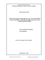
be more complex. A practical circuit for checking a (
7
,
4
) SECSED code is
given in Wakerly [p.
298
,
1990
] and is reproduced in Fig.
2
.
7
. For the reader
who is not experienced in digital circuitry, some explanation is in order. The
three
74
LS
280
ICs (U
1

, U
2
, and U
3
) are similar to the SN
74180
shown in Fig.
2
.
4
. Substituting Eq. (
2
.
22
a) into Eq. (
2
.
24
a) shows that the syndrome bit e
1
is dependent on the ⊕ of c
1
, b
1
, b
2
, and b
4
, and from Table
2

.
6
we see that
these are bit positions x
1
, x
3
, x
5
, and x
7
, which correspond to the inputs to
U
1
. Similarly, U
2
and U
3
compute e
2
and e
3
. The decoder U
4
(see Appendix
C
6
.
3
) activates one of its

8
outputs, which is the address of the error bit. The
8
output gates (U
5
and U
6
) are exclusive or gates (see Appendix C; only
7
are
used). The output of the U
4
selects the erroneous bit from the bus DU(
1
–
7
),
complements it (performing a correction), and passes through the other
6
bits
unchanged. Actually the outputs DU(
1
–
7
) are all complements of the desired
values; however, this is simply corrected by a group of inverters at the output
or inversion of the next stage of digital logic. For a check-bit generator, we
can use three
74
LS

280
chips to generate e
1
, e
2
, and e
3
.
We can compute the reliability of the generator
/
checker circuitry by again
using the IC failure rate model of Section B
3
.
3
, l
b

0
.
004

g . We assume
54
CODING TECHNIQUES
74LS86
74LS86
74LS86
74LS86
74LS86

74LS86
74LS86
DU1
DU2
DU3
DU4
DU5
DU6
DU7
1
4
10
13
1
4
10
2
5
9
12
2
5
9
/E1
/E2
/E3
/E4
/E5
/E6
/E7

3
6
8
11
3
6
8
/DC1
/DC2
/DC3
/DC4
/DC5
/DC6
/DC7
U5
U5
U5
U5
U6
U6
U6
U4
/DC[1–7]
/NO ERROR
15
14
13
12
11
10

9
7
Y0
Y1
Y2
Y3
EVEN
EVEN
EVEN
ODD
ODD
ODD
Y4
Y5
Y6
Y7
G1
G2A
G2B
A
A
A
A
B
B
B
B
C
C
C

C
D
D
D
E
E
E
F
F
F
G
G
G
H
H
H
I
I
I
+5V
R
74LS138
74LS280
74LS280
74LS280
6
4
5
1
2

3
SYN0
SYN1
SYN2
5
5
5
6
6
6
DU[1–7]
8
8
8
DU7
DU7
DU7
DU5
DU6
DU6
DU3
DU3
DU5
DU1
DU2
DU4
9
9
9
10

10
10
11
11
11
12
12
12
13
13
13
1
1
1
2
2
2
4
4
4
U1
U2
U3
Figure
2
.
7
Error-correcting circuit for a Hamming (
7
,

4
) SECSED code [Reprinted
by permission of Pearson Education, Inc., Upper Saddle River, NJ
07458
; from Wak-
erly,
2000
, p.
298
].
that any failure in the IC causes system failure, so the reliability diagram is a
series structure and the failure rates add. The computation is detailed in Table
2
.
12
. (See also Fig.
2
.
7
.)
Thus the failure rate for the coder plus decoder is l

13
.
58
×
10
−
8
, which

is about four times as large as that for the parity bit case (
2
×
1
.
67
×
10
−
8
)
that was calculated previously.
We now incorporate the possibility of generator
/
checker failure and how it
affects the error-correction performance in the same manner as we did with the
parity-bit code in Eqs. (
2
.
8
)–(
2
.
11
). From Table
2
.
8
we see that a
1

-byte (
8
-bit)
message requires
4
check bits; thus the SECSED code is (
12
,
8
). The example
developed in Table
2
.
12
and Fig.
2
.
7
was for a (
7
,
4
) code, but we can easily
modify these results for the (
12
,
8
) code we have chosen to discuss. First, let
us consider the code generator. The
74

LS
280
chips are designed to generate
parity check bits for up to an
8
-bit word, so they still suffice; however, we now