Tài liệu Độ tin cậy của hệ thống máy tính và mạng P6 ppt

6
NETWORKED SYSTEMS
RELIABILITY
Reliability of Computer Systems and Networks: Fault Tolerance, Analysis, and Design
Martin L. Shooman
Copyright 
2002
John Wiley & Sons, Inc.
ISBNs:
0
-
471
-
29342
-
3
(Hardback);
0
-
471
-
22460
-X (Electronic)
283
6
.
1
INTRODUCTION
Many physical problems (e.g., computer networks, piping systems, and power
grids) can be modeled by a network. In the context of this chapter, the word
network means a physical problem that can be modeled as a mathematical

graph composed of nodes and links (directed or undirected) where the branches
have associated physical parameters such as flow per minute, bandwidth, or
megawatts. In many such systems, the physical problem has sources and sinks
or inputs and outputs, and the proper operation is based on connection between
inputs and outputs. Systems such as computer or communication networks have
many nodes representing the users or resources that desire to communicate and
also have several links providing a number of interconnected pathways. These
many interconnections make for high reliability and considerable complexity.
Because many users are connected to such a network, a failure affects many
people; thus the reliability goals must be set at a high level.
This chapter focuses on computer networks. It begins by discussing the sev-
eral techniques that allow one to analyze the reliability of a given network, after
which the more difficult problem of optimum network design is introduced.
The chapter concludes with a brief introduction to one of the most difficult
cases to analyze—where links can be disabled because of two factors: (a) link
congestion (a situation in which flow demand exceeds flow capacity and a link
is blocked or an excessive queue builds up at a node), and (b) failures from
broken links.
A new approach to reliability in interconnected networks is called surviv-
ability analysis [Jia and Wing,
2001
]. The concept is based on the design of
284
NETWORKED SYSTEMS RELIABILITY
a network so it is robust in the face of abnormal events—the system must
survive and not crash. Recent research in this area is listed on Jeannette M.
Wing’s Web site [Wing,
2001
].
The mathematical techniques used in this chapter are properties of mathe-

matical graphs, tie sets, and cut sets. A summary of the relevant concepts is
given in Section B
2
.
7
, and there is a brief discussion of some aspects of graph
theory in Section
5
.
3
.
5
; other concepts will be developed in the body of the
chapter. The reader should be familiar with these concepts before continuing
with this chapter. For more details on graph theory, the reader is referred to
Shooman [
1983
, Appendix C]. There are of course other approaches to net-
work reliability; for these, the reader is referred to the following references:
Frank [
1971
], Van Slyke [
1972
,
1975
], and Colbourn [
1987
,
1993
,

1995
]. It
should be mentioned that the cut-set and tie-set methods used in this chapter
apply to reliability analyses in general and are employed throughout reliabil-
ity engineering; they are essentially a theoretical generalization of the block
diagram methods discussed in Section B
2
. Another major approach is the
use of fault trees, introduced in Section B
5
and covered in detail in Dugan
[
1996
].
In the development of network reliability and availability we will repeat for
clarity some of the concepts that are developed in other chapters of this book,
and we ask for the reader’s patience.
6
.
2
GRAPH MODELS
We focus our analytical techniques on the reliability of a communication net-
work, although such techniques also hold for other network models. Suppose
that the network is composed of computers and communication links. We rep-
resent the system by a mathematical graph composed of nodes representing the
computers and edges representing the communications links. The terms used to
describe graphs are not unique; oftentimes, notations used in the mathematical
theory of graphs and those common in the application fields are interchange-
able. Thus a mathematics textbook may talk of vertices and arcs; an electrical-
engineering book, of nodes and branches; and a communications book, of sites

and interconnections or links. In general, these terms are synonymous and used
interchangeably.
In the most general model, both the nodes and the links can fail, but here
we will deal with a simplified model in which only the links can fail and the
nodes are considered perfect. In some situations, communication can go only
in one direction between a node pair; the link is represented by a directed edge
(an arrowhead is added to the edge), and one or more directed edges in a graph
result in a directed graph (digraph). If communication can occur in both direc-
tions between two nodes, the edge is nondirected, and a graph without any
directed nodes is an ordinary graph (i.e., nondirected, not a digraph). We will
consider both directed and nondirected graphs. (Sometimes, it is useful to view
DEFINITION OF NETWORK RELIABILITY
285
ab1
42
dc3
5
6
Figure
6
.
1
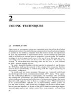
A four-node graph representing a computer or communication network.
a nondirected graph as a special case of a directed graph in which each link
is represented by two identical parallel links, with opposite link directions.)
When we deal with nondirected graphs composed of E edges and N nodes,
the notation G(N, E) will be used. A particular node will be denoted as n
i
and
a particular edge denoted as e

j
. We can also identify an edge by naming the
nodes that it connects; thus, if edge j is between nodes s and t, we may write
e
j

(n
s
, n
t
)

e(s, t). One also can say that edge j is incident on nodes s and
t. As an example, consider the graph of Fig.
6
.
1
, where G(N

4
, E

6
). The
nodes n
1
, n
2
, n
3

, and n
4
are a, b, c, and d. Edge
1
is denoted by e
1

e(n
1
, n
2
)

(a, b), edge
2
by e
2

e(n
2
, n
3
)

(b, c), and so forth. The example of a network
graph shown in Fig.
6
.
1
has four nodes (a, b, c, d) and six edges (

1
,
2
,
3
,
4
,
5
,
6
). The edges are undirected (directed edges have arrowheads to show the
direction), and since in this particular example all possible edges between the
four nodes are shown, it is called a complete graph. The total number of edges
in a graph with n nodes is the number of combinations of n things taken two
at a time

n!
/
[(
2
!)(n −
2
)!]. In the example of Fig.
6
.
1
, the total number of
edges in
4

!
/
[(
2
!)(
4
−
2
)!]

6
.
In formulating the network model, we will assume that each link is either
good or bad and that there are no intermediate states. Also, independence of
link failures is assumed, and no repair or replacement of failed links is con-
sidered. In general, the links have a high reliability, and because of all the
multiple (redundant) paths, the network has a very high reliability. This large
number of parallel paths makes for high complexity; the efficient calculation
of network reliability is a major problem in the analysis, design, or synthesis
of a computer communication network.
6
.
3
DEFINITION OF NETWORK RELIABILITY
In general, the definition of reliability is the probability that the system oper-
ates successfully for a given period of time under environmental conditions
(see Appendix B). We assume that the systems being modeled operate con-
tinuously and that the time in question is the clock time since the last failure
286
NETWORKED SYSTEMS RELIABILITY

or restart of the system. The environmental conditions include not only tem-
perature, atmosphere, and weather, but also system load or traffic. The term
successful operation can have many interpretations. The two primary ones are
related to how many of the n nodes can communicate with each other. We
assume that as time increases, a number of the m links fail. If we focus on
communication between a pair of nodes where s is the source node and t is
the target node, then successful operation is defined as the presence of one or
more operating paths between s and t. This is called the two-terminal problem,
and the probability of successful communication between s and t is called two-
terminal reliability. If successful operation is defined as all nodes being able
to communicate, we have the all-terminal problem, for which it can be stated
that node s must be able to communicate with all the other n −
1
nodes, since
communication between any one node s and all others nodes, t
1
, t
2
, . . . , t
n −
1
,
is equivalent to communication between all nodes. The probability of success-
ful communication between node s and nodes t
1
, t
2
, . . . , t
n −
1

is called the all-
terminal reliability.
In more formal terms, we can state that the all-terminal reliability is the
probability that node n
i
can communicate with node n
j
for all pairs n
i
n
j
(where
i
϶
j ). We wish to show that this is equivalent to the proposition that node s
can communicate with all other nodes t
1

n
2
, t
2

n
3
, . . . , t
n −
1

n

n
. Choose
any other node n
x
(where x
϶
1
). By assumption, n
x
can communicate with s
because s can communicate with all nodes and communication is in both direc-
tions. However, once n
x
reaches s, it can then reach all other nodes because
s is connected to all nodes. Thus all-terminal connectivity for x

1
results in
all-terminal connectivity for x
϶
1
, and the proposition is proved.
In general, reliability, R, is the probability of successful operation. In the
case of networks, we are interested in all-terminal reliability, R
all
:
R
all

P(that all n nodes are connected) (

6
.
1
)
or the two-terminal reliability:
R
st

P(that nodes s and t are connected) (
6
.
2
)
Similarly, k-terminal reliability is the probability that a subset of k nodes
2
≤
k ≤ n) are connected. Thus we must specify what type of reliability we are
discussing when we begin a problem.
We stated previously that repairs were not included in the analysis of net-
work reliability. This is not strictly true; for simplicity, no repair was assumed.
In actuality, when a node-switching computer or a telephone communications
line goes down, each is promptly repaired. The metric used to describe a
repairable system is availability, which is defined as the probabilty that at any
instant of time t, the system is up and available. Remember that in the case
of reliability, there were no failures in the interval
0
to t. The notation is A(t),
and availability and reliability are related as follows by the union of events:
DEFINITION OF NETWORK RELIABILITY
287

A(t)

P(no failure in interval
0
to t +
1
failure and
1
repair in interval
0
to t +
2
failures and
2
repairs in interval
0
to t + · · ·) (
6
.
3
)
The events in Eq. (
6
.
3
) are all mutually exclusive; thus Eq. (
6
.
3
) can be

expanded as a sum of probabilities:
A(t)

P(no failure in interval
0
to t)
+ P(
1
failure and
1
repair in interval
0
to t)
+ P(
2
failures and
2
repairs in interval
0
to t)+·· · (
6
.
4
)
Clearly,
•
The first term in Eq. (
6
.
4

) is the reliability, R(t)
•
A(t)

R(t)

1
at t

0
•
For t >
0
, A(t) > R(t)
•
R(t) 
0
as t  ∞
•
It is shown in Appendix B that A(t)  A
ss
as t  ∞ and, as long as repair
is present, A
ss
>
0
Availability is generally derived using Markov probability models (see
Appendix B and Shooman [
1990
]). The result of availability derivations for

a single element with various failure and repair probability distributions can
become quite complex. In general, the derivations are simplified by assuming
exponential probability distributions for the failure and repair times (equiv-
alent to constant-failure rate, l, and constant-repair rate, m). Sometimes, the
mean time to failure (MTTF) and the mean time to repair (MTTR) are used
to describe the repair process and availability. In many cases, the terms mean
time between failure (MTBF) and mean time between repair (MTBR) are used
instead of MTTF and MTTR. For constant-failure and -repair rates, the mean
times become MTBF

1
/
l and MTBR

1
/
m. The solution for A(t) has an
exponentially decaying transient term and a constant steady-state term. After a
few failure repair cycles, the transient term dies out and the availability can be
represented by the simpler steady-state term. For the case of constant-failure
and -repair rates for a single item, the steady-state availability is given by the
equation that follows (see Appendix B).
A
ss

m
/
(l + m)

MTBF

/
(MTBF + MTBR) (
6
.
5
)
Since the MTBF >> MTBR in any well-designed system, A
ss
is close to
unity. Also, alternate definitions for MTTF and MTTR lead to slightly different
but equivalent forms for Eq. (
6
.
5
) (see Kershenbaum [
1993
].)
Another derivation of availability can be done in terms of system uptime,
U(t), and system downtime, D(t), resulting in the following different formula
for availability:
288
NETWORKED SYSTEMS RELIABILITY
A
ss

U(t)
/
[U(t) + D(t)] (
6
.

6
)
The formulation given in Eq. (
6
.
6
) is more convenient than that of Eq. (
6
.
5
)
if we wish to estimate A
ss
based on collected field data. In the case of a com-
puter network, the availability computations can become quite complex if the
repairs of the various elements are coupled, in which case a single repairman
might be responsible for maintaining, say, two nodes and five lines. If sev-
eral failures occur in a short period of time, a queue of failed items wait-
ing for repairs might build up and the downtime is lengthened, and the term
“repairman-coupled” is used. In the ideal case, if we assume that each element
in the system has its own dedicated repairman, we can guarantee that the ele-
ments are decoupled and that the steady-state availabilities can be substituted
into probability expressions in the same way as reliabilities are. In a practi-
cal case, we do not have individual repairmen, but if the repair rate is much
larger than the failure rate of the several components for which the repairman
supports, then approximate decoupling is a good assumption. Thus, in most
network reliability analyses there will be no distinction made between reli-
ability and availability; the two terms are used interchangeably in the network
field in a loose sense. Thus a reliability analyst would make a combinatorial
model of a network and insert reliability values for the components to calculate

system reliability. Because decoupling holds, he or she would substitute com-
ponent availabilities in the same model and calculate the system availability;
however, a network analyst would perform the same availability computation
and refer to it colloquially as “system reliability.” For a complete discussion
of availability, see Shooman [
1990
].
6
.
4
TWO-TERMINAL RELIABILITY
The evaluation of network reliability is a difficult problem, but there are several
approaches. For any practical problem of significant size, one must use a com-
putational program. Thus all the techniques we discuss that use a “pencil-paper-
and-calculator” analysis are preludes to understanding how to write algorithms
and programs for network reliability computation. Also, it is always valuable to
have an analytical solution of simpler problems for use to test reliability com-
putation programs until the user becomes comfortable with such a program.
Since two-terminal reliability is a bit simpler than all-terminal reliability, we
will discuss it first and treat all-terminal reliability in the following section.
6
.
4
.
1
State-Space Enumeration
Conceptually, the simplest means of evaluating the two-terminal reliability of
a network is to enumerate all possible combinations where each of the e edges
can be good or bad, resulting in
2

e
combinations. Each of these combinations of
good and bad edges can be treated as an event E
i
. These events are all mutually
TWO-TERMINAL RELIABILITY
289
exclusive (disjoint), and the reliability expression is simply the probability of
the union of the subset of these events that contain a path between s and t.
R
st

P(E
1
+ E
2
+ E
3
·· ·) (
6
.
7
)
Since each of these events is mutually exclusive, the probability of the union
becomes the sum of the individual event probabilities.
R
st

P(E
1

) + P(E
2
) + P(E
3
) + · · · (
6
.
8
)
[Note that in Eq. (
6
.
7
) the symbol + stands for union (
U
), whereas in Eq. (
6
.
8
),
the + represents addition. Also throughout this chapter, the intersection of x and
y (x
U
y) is denoted by x
.
y, or just xy.]
As an example, consider the graph of a complete four-node communication
network that is shown in Fig.
6
.

1
. We are interested in the two-terminal reli-
ability for node pair a and b; thus s

a and t

b. Since there are six edges,
there are
2
6

64
events associated with this graph, all of which are presented
in Table
6
.
1
. The following definitions are used in constructing Table
6
.
1
:
E
i

the event i
j

the success of edge j
j

′

the failure of edge j
The term good means that there is at least one path from a to b for the given
combination of good and failed edges. The term bad, on the other hand, means
that there are no paths from a to b for the given combination of good and failed
edges. The result—good or bad—is determined by inspection of the graph.
Note that in constructing Table
6
.
1
, the following observations prove help-
ful: Any combination where edge
1
is good represents a connection, and at
least three edges must fail (edge
1
plus two others) for any event to be bad.
Substitution of the good events from Table
6
.
1
into Eq. (
6
.
8
) yields the
two-terminal reliability from a to b:
R
ab


[P(E
1
)] + [P(E
2
) +·· ·+P(E
7
)] + [P(E
8
) + P(E
9
) + · · · + P(E
22
)]
+ [P(E
23
)+P(E
24
) + · · · + P(E
34
) + P(E
37
) + · · · + P(E
42
)]
+ [P(E
43
)+P(E
44
) + · · · + P(E

47
) + P(E
50
) + P(E
56
)] + [P(E
58
)] (
6
.
9
)
The first bracket in Eq. (
6
.
9
) has one term where all the edges must be good,
and if all edges are identical and independent, and they have a probability of
success of p, then the probability of event E
1
is p
6
. Similarly, for the second
bracket, there are six events of probability qp
5
where the probability of failure
q

1
− p, etc. Substitution in Eq. (

6
.
9
) yields a polynomial in p and q:
R
ab

p
6
+
6
qp
5
+
15
q
2
p
4
+
18
q
3
p
3
+
7
q
4
p

2
+ q
5
p (
6
.
10
)
290
NETWORKED SYSTEMS RELIABILITY
TABLE
6
.
1
The Event-Space for the Graph of
Fig.
6
.
1
(s

a, t

b)
No failures:
΂
6
0
΃


6
!
0
!
6
!

1
E
1

123456
Good
One failure:
΂
6
1
΃

6
!
1
!
5
!

6
E
2


1
′
23456
Good
E
3

12
′
3456
Good
E
4

123
′
456
Good
E
5

1234
′
56
Good
E
6

12345
′

6
Good
E
7

123456
′
Good
Two failures:
΂
6
2
΃

6
!
2
!
4
!

15
E
8

1
′
2
′
3456

Good
E
9

1
′
23
′
456
Good
E
10

1
′
234
′
56
Good
E
11

1
′
2345
′
6
Good
E
12


1
′
23456
′
Good
E
13

12
′
3
′
456
Good
E
14

12
′
34
′
56
Good
E
15

12
′
345

′
6
Good
E
16

12
′
3456
′
Good
E
17

123
′
4
′
56
Good
E
18

123
′
45
′
6
Good
E

19

123
′
456
′
Good
E
20

1234
′
5
′
6
Good
E
21

1234
′
56
′
Good
E
22

12345
′
6

′
Good
Continued . . .
Three failures:
΂
6
3
΃

6
!
3
!
3
!

20
E
23

1234
′
5
′
6
′
Good
E
24


123
′
45
′
6
′
Good
E
25

123
′
4
′
56
′
Good
E
26

123
′
4
′
5
′
6
Good
E
27


12
′
345
′
6
′
Good
E
28

12
′
34
′
56
′
Good
E
29

12
′
34
′
5
′
6
Good
E

30

12
′
3
′
456
′
Good
E
31

12
′
3
′
45
′
6
Good
E
32

12
′
3
′
4
′
56

Good
TWO-TERMINAL RELIABILITY
291
TABLE
6
.
1
(Continued)
E
33

1
′
2345
′
6
′
Good
E
34

1
′
234
′
56
′
Good
E
35


1
′
234
′
5
′
6
′
Bad
E
36

1
′
2
′
3456
′
Bad
E
37

1
′
2
′
345
′
6

Good
E
38

1
′
2
′
34
′
56
Good
E
39

1
′
23
′
456
′
Good
E
40

1
′
23
′
45

′
6
Good
E
41

1
′
23
′
4
′
56
Good
E
42

1
′
2
′
3
′
456
Good
Four failures:
΂
6
4
΃


6
!
4
!
2
!

15
E
43

123
′
4
′
5
′
6
′
Good
E
44

12
′
34
′
5
′

6
′
Good
E
45

12
′
3
′
45
′
6
′
Good
E
46

12
′
3
′
4
′
56
′
Good
E
47


12
′
3
′
4
′
5
′
6
Good
E
48

1
′
234
′
5
′
6
′
Bad
E
49

1
′
23
′
45

′
6
′
Bad
E
50

1
′
23
′
4
′
56
′
Good
E
51

1
′
23
′
4
′
5
′
6
Bad
E

52

1
′
2
′
345
′
6
′
Bad
E
53

1
′
2
′
34
′
56
′
Bad
E
54

1
′
2
′

34
′
5
′
6
Bad
E
55

1
′
2
′
3
′
456
′
Bad
E
56

1
′
2
′
3
′
45
′
6

Good
E
57

1
′
2
′
3
′
4
′
56
Bad
Continued . . .
Five failures:
΂
6
5
΃

6
!
5
!
1
!

6
E

58

12
′
3
′
4
′
5
′
6
′
Good
E
59

1
′
23
′
4
′
5
′
6
′
Bad
E
60


1
′
2
′
34
′
5
′
6
′
Bad
E
61

1
′
2
′
3
′
45
′
6
′
Bad
E
62

1
′

2
′
3
′
4
′
56
′
Bad
E
63

1
′
2
′
3
′
4
′
5
′
6
Bad
Six failures:
΂
6
6
΃


6
!
6
!
0
!

1
E
64

1
′
2
′
3
′
4
′
5
′
6
′
Bad
Substitutions such as those in Eq. (
6
.
10
) are prone to algebraic mistakes; as
a necessary (but not sufficient) check, we evaluate the polynomial for p


1
and q

0
, which should yield a reliability of unity. Similarly, evaluating the
292
NETWORKED SYSTEMS RELIABILITY
polynomial for p

0
and q

1
should yield a reliability of
0
. (Any network
has a reliability of unity regardless of its topology if all edges are perfect; it
has a reliability of
0
if all its edges have failed.)
Numerical evaluation of the polynomial for p

0
.
9
and q

0
.

1
yields
R
ab

0
.
9
6
+
6
(
0
.
1
)(
0
.
9
)
5
+
15
(
0
.
1
)
2
(

0
.
9
)
4
+
18
(
0
.
1
)
3
(
0
.
9
)
3
+
7
(
0
.
1
)
4
(
0
.

9
)
2
+ (
0
.
1
)
5
(
0
.
9
)(
6
.
11
a)
R
ab

0
.
5314
+
0
.
35427
+
0

.
0984
+
0
.
0131
+
5
.
67
×
10
−
4
+
9
×
10
−
6
(
6
.
11
b)
R
ab

0
.

997848
(
6
.
11
c)
Usually, event-space-reliability calculations require much effort and time even
though the procedure is clear. The number of events builds up exponentially
as
2
e
. For e

10
, we have
1
,
024
terms, and if we double the e, there are over
a million terms. However, we seek easier methods.
6
.
4
.
2
Cut-Set and Tie-Set Methods
One can reduce the amount of work in a network reliability analysis below the
2
e
complexity required for the event-space method if one focuses on the min-

imal cut sets and minimal tie sets of the graph (see Appendix B and Shooman
[
1990
, Section
3
.
6
.
5
]). The tie sets are the groups of edges that form a path
between s and t. The term minimal implies that no node or edge is traversed
more than once, but another way of defining this is that minimal tie sets have
no subsets of edges that are a tie set. If there are i tie sets between s and t,
then the reliability expression is given by the expansion of
R
st

P(T
1
+ T
2
+ · · · + T
i
)(
6
.
12
)
Similarly, one can focus on the minimal cut sets of a graph. A cut set is a
group of edges that break all paths between s and t when they are removed

from the graph. If a cut set is minimal, no subset is also a cut set. The reliability
expression in terms of the j cut sets is given by the expansion of
R
st

1
− P(C
1
+ C
2
+·· ·+C
j
)(
6
.
13
)
We now apply the above theory to the example given in Fig.
6
.
1
. The min-
imal cut sets and tie sets are found by inspection for s

a and t

b and are
given in Table
6
.

2
.
Since there are fewer cut sets, it is easier to use Eq. (
6
.
13
) rather than Eq.
(
6
.
12
); however, there is no general rule for when j < i or vice versa.
TWO-TERMINAL RELIABILITY
293
TABLE
6
.
2
Minimal Tie Sets and Cut Sets for the
Example of Fig.
6
.
1
(s

a, t

b)
Tie Sets
Cut Sets

T
1

1
C
1

1
′
4
′
5
′
T
2

52
C
2

1
′
6
′
2
′
T
3

46

C
3

1
′
5
′
6
′
3
′
T
4

234
C
4

1
′
2
′
3
′
4
′
T
5

536

—
R
ab

1
− P(C
1
+ C
2
+ C
3
+ C
4
)(
6
.
14
a)
R
ab

1
− P(
1
′
4
′
5
′
+

1
′
6
′
2
′
+
1
′
5
′
3
′
6
′
+
1
′
2
′
3
′
4
′
)(
6
.
14
b)
R

ab

1
− [P(
1
′
4
′
5
′
) + P(
1
′
6
′
2
′
) + P(
1
′
5
′
3
′
6
′
) + P(
1
′
2

′
3
′
4
′
)]
+ [P(
1
′
2
′
4
′
5
′
6
′
)+P(
1
′
3
′
4
′
5
′
6
′
) + P(
1

′
2
′
3
′
4
′
5
′
)
+ P(
1
′
2
′
3
′
5
′
6
′
)+P(
1
′
2
′
3
′
4
′

6
′
) + P(
1
′
2
′
3
′
4
′
5
′
6
′
)]
− [P(
1
′
2
′
3
′
4
′
5
′
6
′
)+P(

1
′
2
′
3
′
4
′
5
′
6
′
) + P(
1
′
2
′
3
′
4
′
5
′
6
′
)
+ P(
1
′
2

′
3
′
4
′
5
′
6
′
)] + [P(
1
′
2
′
3
′
4
′
5
′
6
′
)] (
6
.
14
c)
The expansion of the probability of a union of events that occurs in Eq. (
6
.

14
)
is often called the inclusion–exclusion formula. [See Eq. (A
11
).]
Note that in the expansions in Eqs. (
6
.
12
) or (
6
.
13
), ample use is made of
the theorems x
.
x

x and x +x

x (see Appendix A). For example, the second
bracket in Eq. (
6
.
14
c) has as its second term P(c
1
c
3
)


P([
1
′
4
′
5
′
][
1
′
5
′
6
′
3
′
])

P(
1
′
3
′
4
′
5
′
6
′

), since
1
′
.
1
′

1
′
and
5
′
.
5
′

5
′
. The reader should note that
this point is often overlooked (see Appendix D, Section D
3
), and it may or
may not make a numerical difference.
If all the edges have equal probabilities of failure

q and are independent,
Eq. (
6
.
14

c) becomes
R
ab

1
− [
2
q
3
+
2
q
4
] + [
5
q
5
+ q
6
] − [
4
q
6
] + [q
6
]
R
ab

1

−
2
q
3
−
2
q
4
+
5
q
5
−
2
q
6
(
6
.
15
)
The necessary checks, R
ab

1
for q

0
and R
ab


0
for q

1
, are valid.
For q

0
.
1
, Eq. (
6
.
15
) yields
R
ab

1
−
2
×
0
.
1
3
−
2
×

0
.
1
4
+
5
×
0
.
1
5
−
2
×
0
.
1
6

0
.
997848
(
6
.
16
)
Of course, the result of Eq. (
6
.

16
) is identical to Eq. (
6
.
11
c). If we substitute
tie sets into Eq. (
6
.
12
), we would get a different though equivalent expression.
The expansion of Eq. (
6
.
13
) has a complexity of
2
j
and is more complex
than Eq. (
6
.
12
) if there are more cut sets than tie sets. At this point, it would
294
NETWORKED SYSTEMS RELIABILITY
seem that we should analyze the network and see how many tie sets and cut
sets exist between s and t, and assuming that i and j are manageable numbers
(as is the case in the example to follow), then either Eq. (
6

.
12
) or Eq. (
6
.
13
)
is feasible. In a very large problem (assume i < j < e), even
2
i
is too large
to deal with, and the approximations of Section
6
.
4
.
3
are required. Of course,
large problems will utilize a network reliability computation program, but an
approximation can be used to check the program results or to speed up the
computation in a truly large problem [Colbourn,
1987
,
1993
; Shooman,
1990
].
The complexity of the cut-set and tie-set methods depends on two factors:
the order of complexity involved in finding the tie sets (or cut sets) and the
order of complexity for the inclusion–exclusion expansion. The algorithms for

finding the number of cut sets are of polynomial complexity; one discussed in
Shier [
1991
, p.
63
] is of complexity order O(n + e + ie). In the case of cut sets,
the finding algorithms are also of polynomial complexity, and Shier [
1991
, p.
69
] discusses one that is of order O([n + e] j). Observe that the notation O( f )
is called the order of f or “big O of f.” For example, if f

5
x
3
+
10
x
2
+
12
, the
order of f would be the dominating term in f as x becomes large, which is
5
x
3
.
Since the constant
5

is a multiplier independent of the size of x, it is ignored,
so O(
5
x
3
+
10
x
2
+
12
)

x
3
(see Rosen [
1999
, p.
105
]).
In both cases, the dominating complexity is that of expansion for the
inclusion–exclusion algorithm for Eqs. (
6
.
12
) and (
6
.
13
), where the orders of

complexity are exponential, O(
2
i
) or O(
2
j
) [Colbourn,
1987
,
1993
]. This is
the reason why approximate methods are discussed in the next two sections.
In addition, some of these algorithms are explored in the problems at the end
of this chapter.
If we examine Eqs. (
6
.
12
) and (
6
.
13
), we see that the complexity of
these expressions is a function of the cut sets or tie sets, the number of
edges in the cut sets or tie sets, and the number of “brackets” that must be
expanded (the number of terms in the union of cut sets or tie sets—i.e., in
the inclusion–exclusion formula). We can approximate the cut-set or tie-set
expression by dropping some of the less-significant brackets of the expansion,
by dropping some of the less-significant cut sets or tie sets, or by both.
6

.
4
.
3
Truncation Approximations
The inclusion–exclusion expansions of Eqs. (
6
.
12
) and (
6
.
13
) sometimes yield
a sequence of probabilities that decrease in size so that many of the higher-
order terms in the sequence can be neglected, resulting in a simpler approxi-
mate formula. These terms are products of probabilities, so if these probabil-
ities are small, the higher-order product terms can be neglected. In the case
of tie-set probabilities, this is when the probabilities of success are small—the
so-called low-reliability region, which is not the region of practical interest.
Cut-set analysis is preferred since this is when the probabilities of failure are
small—the so-called high-reliability region, which is really the region of prac-
tical interest. Thus cut-set approximations are the ones most frequently used
TWO-TERMINAL RELIABILITY
295
in practice. If only the first bracket in Eq. (
6
.
14
c) is retained in addition to the

unity term, one obtains the same expression that would have ensued had the
cuts been disjoint (but they are not). Thus we will call the retention of only
the first two terms the disjoint approximation.
In Shooman [
1990
, Section
3
.
6
.
5
], it is shown that a disjoint cut-set approx-
imation is a lower bound. For the example of Fig.
6
.
1
, we obtain Eq. (
6
.
17
)
for the disjoint approximation, and assuming q

0
.
1
:
R
ab
≥

1
− [
2
q
3
+
2
q
4
]

1
−
0
.
002
−
0
.
0002

0
.
9978
(
6
.
17
)
which is quite close to the exact value given in Eq. (

6
.
16
). If we include the
next bracket in Eq. (
6
.
14
c), we get a closer approximation at the expense of
computing [ j + (
j
2
)]

[ j( j −
1
)
/
2
] terms.
R
ab
≤
1
− [
2
q
3
+
2

q
4
] + [
5
q
5
+ q
6
]

0
.
9978
+
5
×
0
.
1
5
+
0
.
1
6

0
.
997851
(

6
.
18
)
Equation (
6
.
18
) is not only an approximation but an upper bound. In fact, as
more terms are included in the inclusion–exclusion formula, we obtain a set of
alternating bounds (see Shooman [
1990
, Section
3
.
6
.
5
]). Note that Eq. (
6
.
17
)
is a sharp lower bound and that Eq. (
6
.
18
) is ever sharper, but both equa-
tions effectively bracket the exact result. Clearly, the sharpness of these bounds
increases as q

i

1
− p
i
decreases for the i edges of the graph.
0
.
997800
≤ R
ab
≤
0
.
997851
(
6
.
19
)
We can approximate R
ab
by the midpoint of the two bounds.
R
ab

0
.
997800
+

0
.
997851
2

0
.
9978255
(
6
.
20
)
The accuracy of the preceding approximation can be evaluated by examining
the deviation in the computed probability of failure F
ab

1
− R
ab
. In the region
of high reliability, all the values of R
ab
are very close to unity, and differences
are misleadingly small. Thus, as our error criterion, we will use
% error

|
F
ab

(estimate) − F
ab
(exact)
|
F
ab
(exact)
×
100
(
6
.
21
)
Of course, the numerator of Eq. (
6
.
21
) would be the same if we took the dif-
ferences in the reliabilities. Evaluation of Eq. (
6
.
21
) for the results given in
Eqs. (
6
.
16
) and (
6

.
20
) yields
% error

|
0
.
0021745
−
0
.
002152
|
0
.
002152
×
100
%

1
.
05
(
6
.
22
)
296

NETWORKED SYSTEMS RELIABILITY
Clearly, this approximation is good for this example and will be good in most
cases. Of course, in approximate evaluations of a large network, we do not
know the exact reliability, but we can still approximate Eq. (
6
.
21
) by using
the difference between the two-term and three-term approximations. For the
numerator and the average of the denominator:
% error ≈
|
0
.
002200
−
0
.
002149
|
0
.
0021745
×
100
%

2
.
35

(
6
.
23
)
A moment’s reflection leads to the conclusion that the highest-order approx-
imation will always be the closest and should be used in the denominator of
an error bound. The numerator, on the other hand, should be the difference
between the two highest-order terms. Thus, for our example,
% error ≈
|
0
.
002200
−
0
.
002149
|
0
.
0021749
×
100
%

2
.
37
(

6
.
24
)
Therefore, a practical approach in designing a computer analysis program is
to ask the analyst to input the accuracy he or she desires, then to compute a
succession of bounds involving more and more terms in the expansion of Eq.
(
6
.
13
) at each stage. An equation similar to Eq. (
6
.
24
) would be used for the
last two terms in the computation to determine when to stop computing alter-
nating bounds. The process truncates when the error approximation yields an
estimated value that has a smaller error bound that that of the required error.
We should take note that the complexity of the “one-at-a-time” approximation
is of order j (number of cut sets) and that of the “two-at-a-time” approxima-
tion is of order j
2
. Thus, even if the error approximation indicates that more
terms are needed, the complexity will only be of order j
3
or perhaps j
4
. The
inclusion–exclusion complexity is therefore reduced from order

2
j
to a poly-
nomial in j (perhaps j
2
or j
3
).
6
.
4
.
4
Subset Approximations
In the last section, we discussed approximation by truncating the inclusion–
exclusion expression. Now we discuss approximation by exclusion of low-
probability cut sets or tie sets. Clearly, the occurrence probability of the lower-
order (fewer edges) cut sets is higher than the higher-order (more edges) ones.
Thus, we can approximate Eq. (
6
.
14
a) dropping C
3
and C
4
fourth-order cut
sets and retaining the third-order cut set to yield an upper bound (since we
have dropped cut sets, we are making an optimistic approximation).
R

ab
≤
1
− P(C
1
+ C
2
)

1
− P(C
1
) − P(C
2
) + P(C
1
)P(C
2
)

1
− P(
1
′
4
′
5
′
) − P(
1

′
6
′
2
′
) + P(
1
′
2
′
4
′
5
′
6
′
)(
6
.
25
a)
For q

0
.
1
,
TWO-TERMINAL RELIABILITY
297
R

ab
≤
1
−
2
×
0
.
1
3
+
0
.
1
5

0
.
99801
(
6
.
25
b)
We can use similar reasoning to develop a lower bound (we drop tie sets,
thereby making a pessimistic approximation) by dropping all but the “one-
hop” tie sets (T
1
) and the “two-hop” tie sets (T
2

, T
3
)—compare Eq. (
6
.
12
) and
Table
6
.
2
.
R
ab
≥ P(T
1
+ T
2
+ T
3
)

P(
1
+
25
+
46
)


P(
1
)+P(
25
) + P(
46
)
− [P(
125
)+P(
146
) + P(
2456
)] + [P(
12456
)] (
6
.
26
a)
For p

0
.
9
,
R
ab
≥ p +
2

p
2
−
2
p
3
− p
4
+ p
5

0
.
9
+
2
×
0
.
9
2
−
2
×
0
.
9
3
−
0

.
9
4
+
0
.
9
5

0
.
99639
(
6
.
26
b)
Given Eq. (
6
.
25
b) and (
6
.
26
b), we can bound R
ab
by
0
.

99639
≤ R
ab
≤
0
.
99801
(
6
.
27
)
and approximate R
ab
by the midpoint of the two bounds:
R
ab

0
.
99639
+
0
.
99801
2

0
.
9971955

(
6
.
28
)
The error bound for this approximation is computed in the same manner as
Eq. (
6
.
23
).
% error ≈
|
0
.
00361
−
0
.
00199
|
0
.
0028045
×
100
%

57
.

8
(
6
.
29
)
The percentage error is larger than in the case of the truncation approxima-
tions, but it remains small enough for the approximation to be valid. The com-
plexity is still exponential—of order
2
x
; however, x is now a small integer and
2
x
is of modest size. Furthermore, the tie-set and cut-set algorithms take less
time since we now do not need to find all cut sets and tie sets—only those of
order ≤ x. Of course, one can always combine both approximation methods by
dropping out higher-order cut sets and then also truncating the expansion. For
more details on network reliability approximations, see Murray [
1992
,
1993
].
6
.
4
.
5
Graph Transformations
Anyone who has studied electric-circuit theory in a physics or engineering

class knows that complex networks of resistors can be reduced to an equiva-
lent single resistance through various combinations of series, parallel, and Y–D
transformations. Such knowledge has obviously stimulated the development
298
NETWORKED SYSTEMS RELIABILITY
(a) Series: PP
ac
= (1 • 2)
PP
ab
= (1 + 2)
=
=
12
abc
1 • 2
1 + 2
a
a
a
c
c
b
(b) Parallel:
(c) Decomposition
(Edge Factoring):
a
c
b
d

1
3
2
4
5
Expand about 5: = [ (5) ( ) + (5 ) ( )]R P Pr G P Pr G
ad 12
’
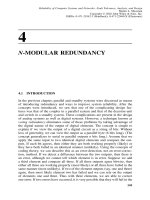
Figure
6
.
2
Illustration of series, parallel, and decomposition transformations for two-
terminal pair networks.
of equivalent network transformations: some that are remarkably similar, and
some that are quite different, especially in the case of all-terminal reliability (to
be discussed later). We must remember that these are not flow transformations
but probability transformations.
This method of calculating network reliability is based on transforming the
network into a simpler network (or set of networks) by successively applying
transformations. Such transformations are simpler for two-terminal reliability
than for all-terminal reliability. For example, for two-terminal reliability, we
can use the transformations given in Fig.
6
.
2
. In this figure, the series transfor-
mation indicates that we replace two branches in series with a single branch
that is denoted by the intersection of the two original branches (
1

.
2
). In the
parallel transformation, we replace the two parallel branches with a single-
series branch that is denoted by the union of the two parallel branches (
1
+
2
).
The edge-factoring case is more complex; the obvious branch to factor about is
edge
5
, which complicates the graph. Edge
5
is considered good and has a prob-
ability of
1
(shorted), and the graph decomposes to G
1
. If edge
5
is bad, how-
ever, it is assumed that no transmission can occur and that it has a probability
of
0
(open circuit), and the graph decomposes to G
2
. Note that both G
1
and G

2
can now be evaluated by using combinations of series and parallel transforma-
tions. These three transformations—series, parallel, and decomposition—are
all that is needed to perform the reliability analysis for many networks.
TWO-TERMINAL RELIABILITY
299
Now we discuss a more difficult network configuration. In the first transfor-
mation in Fig.
6
.
2
(a) series, we readily observe that both (intersection) edges
1
and
2
must be up for a connection between a and b to occur. However, this
transformation only works if there is no third edge connected to node b; if
a third edge exists, a more elaborate transformation is needed (which will be
discussed in Section
6
.
6
on all-terminal reliability). Similarly, in the case of
the parallel transformation, nodes a and b are connected if either (union) a or
b is up.
Assume that any failures of edge
1
and edge
2
are independent and the

probabilities of success for edges
1
and
2
are p
1
and p
2
(probabilities of failure
are q
1

1
− p
1
, q
2

1
− p
2
). Then for the series subnetwork of Fig.
6
.
2
(a),
p
ac

p

1
p
2
, and for the parallel subnetwork in Fig.
6
.
2
(b), p
ab

p
1
+ p
2
− p
1
p
2

1
− q
1
q
2
.
The case of decomposition (called the keystone component method in sys-
tem reliability [Shooman,
1990
] or the edge-factoring method in network reli-
ability) is a little more subtle; it is used to eliminate an edge x from a graph.

Since all edges must either be up or down, we reduce the original network to
two other networks G
1
(given that edge x is up) and G
2
(given that edge x is
down). In general, one uses series and parallel transformations first, resorting
to edge-factoring only when no more series or parallel transformations can be
made. In the subnetwork of Fig.
6
.
2
(c), we see that neither series nor parallel
transformation is immediately possible because of edge
5
, for which reason
decomposition should be used.
The mathematical basis of the decomposition transformation lies in the laws
of conditional probability and Bayesian probability [Mendenhall,
1990
, pp.
64
–
65
]. These laws lead to the following probability equation for terminal pair
st and edge x.
P(there is a path between s and t)

P(x is good) × P(there is a path between s and t
|

x is good)
+ P(x is bad) × P(there is a path between s and t
|
x is bad) (
6
.
30
)
The preceding equation can be rewritten in a more compact notation as follows:
P
st

P(x)P(G
1
) + P(x
′
)P(G
2
)(
6
.
31
)
The term P(G
1
) is the probability of a connection between s and t for the
modified network where x is good, that is, the terminals at either end of edge
x are connected to the graph [see Fig.
6
.

2
(c)]. Similarly, the term P(G
2
) is the
probability that there is a connection between s and t for the modified network
G
2
where x is bad, that is, the edge x is removed from the graph [again, see
Fig.
6
.
2
(c)]. Thus Eq. (
6
.
31
) becomes for st

ad:
P
st

p
5
(
1
− q
1
q
3

)(
1
− q
2
q
4
) + q
5
(p
1
p
2
+ p
3
p
4
− p
1
p
2
p
3
p
4
)(
6
.
32
)
300

NETWORKED SYSTEMS RELIABILITY
ab1
42
dc3
5
a b, d1
2
c
5
4
3
G
1
: Edge 6 good (short) G
2
: Edge 6 bad (open)
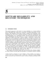
Figure
6
.
3
Decomposition subnetworks for the graph of Fig.
6
.
1
expanded about
edge
6
.
Of course, in most examples, networks G
1

and G
2
are a bit more complex, and
sometimes transformations are recursively computed. More examples of trans-
formations appear in the problems at the end of this chapter; for a complete
discussion of transformations, see Satyanarayana [
1985
] and A. M. Shooman
[
1992
].
We can illustrate the use of the three transformations of Fig.
6
.
2
on the
network given in Fig.
6
.
1
, where we begin by decomposing about edge
6
.
R
ab

P(
6
)
.

P[G
1
]+P(
6
′
)
.
P[G
2
](
6
.
33
)
The networks G
1
and G
2
are shown in Fig.
6
.
3
. Note that for edge
6
good
(up), nodes b and d merge in G
1
, whereas for edge
6
bad (down), edge

6
is
simply removed from the network.
We now calculate P(G
1
) and P(G
2
) for a connection between nodes a and
b with the aid of the series and parallel transformations of Fig.
6
.
2
:
P(G
1
)

P(
1
+
4
+
52
+
53
)

[P(
1
)+P(

4
) + P(
52
) + P(
53
)]
− [P(
14
)+P(
152
) + P(
153
) + P(
452
) + P(
453
) + P(
523
)]
+ [P(
4534
)+P(
1523
) + P(
1453
) + P(
1452
)] − [P(
14523
)] (

6
.
34
)
P(G
2
)

P(
1
+
25
+
243
)

[P(
1
)+P(
25
) + P(
243
)]
− [P(
125
)+P(
1243
) + P(
2543
)] + [P(

12543
)] (
6
.
35
)
Assuming that all edges are identical and independent with probabilities of
success and failure of p and q, substitution into Eqs. (
6
.
33
), (
6
.
34
), and (
6
.
35
)
yields
R
ab

p[
2
p + p
2
−
5

p
3
+
4
p
4
− p
5
] + q[ p + p
2
−
2
p
4
+ p
5
](
6
.
36
)
NODE PAIR RESILIENCE
301
Substitution of p

0
.
9
and q


0
.
1
into Eq. (
6
.
36
) yields
R
ab

0
.
9
[
0
.
99891
] +
0
.
1
[
0
.
98829
]

0
.

997848
(
6
.
37
)
Of course, this result agrees with the previous computation given in Eq. (
6
.
16
).
6
.
5
NODE PAIR RESILIENCE
All-terminal reliability, in which all the node pairs can communicate, is dis-
cussed in the next section. Also, k-terminal reliability will be treated as a speci-
fied subset (
2
≤ k ≤ all-terminal pairs) of all-terminal reliability. In this section,
another metric, essentially one between two-terminal and all-terminal, is dis-
cussed.
Van Slyke and Frank [
1972
] proposed a measure they called resilience for
the expected number of node pairs that can communicate (i.e., they are con-
nected by one or more tie sets). Let s and t represent a node pair. The number
of node pairs in a network with N nodes is the number of combinations of N
choose
2

, that is, the number of combinations of
2
out of N.
Number of node pairs

΂
N
2
΃

N!
2
!(N −
2
)!

N(N −
1
)
2
(
6
.
38
)
Our notation for the set of s, t node pairs contained in an N node network is
{s, t} ⊂ N, and the expected number of node pairs that can communicate is
denoted as resilience, res(G ):
res(G)


Α
Α
Α
{s, t} ⊂ N
R
st
(
6
.
39
)
We can illustrate a resilience calculation by applying Eq. (
6
.
39
) to the net-
work of Fig.
6
.
1
. We begin by observing that if p

0
.
9
for each edge, symmetry
simplifies the computation. The node pairs divide into two categories: the edge
pairs (ab, ad, bc, and cd ) and the diagonal pairs (ac and bd). The edge-pair
reliabilities were already computed in Eqs. (
6

.
36
) and (
6
.
37
). For the diago-
nals, we can use the decomposition given in Fig.
6
.
3
(where s

a and t

c)
and compute R
ac
as shown in the following equations: