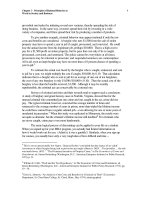
Tài liệu Microeconomics for MBAs 6 doc

Chapter 2 Competitive Product Markets


10
• Change in the profitability of producing other goods
• Change in the scarcity (and prices) of various productive resources
Many other factors, such as weather, can also affect production costs. A change in any of these
determinants of supply can either increase or decrease supply.

• An increase in supply is an increase in the quantity producers are willing and able to
offer at each and every price. It is represented graphically by a rightward, or outward,
shift in the supply curve.
• A decrease in supply is a decrease in the quantity producers are willing and able to
offer at each and every price. It is represented graphically by a leftward, or inward,
shift in the supply curve.


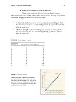
TABLE 2.2 Market Supply of Tomatoes

Price-Quantity
Combinations Price per Bushel Number of Bushels

A $0 0
B 1 10
C 2 20
D 3 30
E 4 40
F 5 50
G 6 60
H 7 70
I 8 80

J 9 90
K 10 100
L 11 110



FIGURE 2.3 Supply of Tomatoes
Supply, the assumed relationship between price
and quantity produced, can be represented by a
curve that slopes up toward the right. Here, as the
price rises from zero to $11, the number of bushels
of tomatoes offered for sale during the course of a
week rises from zero to 110,000.



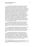
Chapter 2 Competitive Product Markets


11


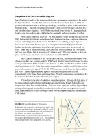
In Figure 2.4, an increase in supply is represented by the shift from S
1
to S
2
. Producers
are willing to produce a larger quantity at each price -- Q
3
instead of Q2 at price P

2
, for
example. They will also accept a lower price for each quantity -- P
1
instead of P2 for quantity
Q
2
. Conversely, the decrease in supply represented by the shift from S
1
to S
3
means that
producers will offer less at each price -- Q
1
instead of Q
2
at price P
2
. They must also have a
higher price for each quantity -- P
3
instead of P
2
for quantity Q
2
.
A few examples will illustrate the impact of changes in the determinants of supply. If
firms learn how to produce more goods with the same or fewer resources, the cost of producing
any given quantity will fall. Because of the technological improvement, firms will be able to offer
a larger quantity at any given price or the same quantity at a lower price. The supply will

increase, shifting the supply curve outward to the right.
Similarly, if the profitability of producing oranges increases relative to grapefruit,
grapefruit producers will shift their resources to oranges. The supply of oranges will increase,
shifting the supply curve to the right. Finally, if lumber (or labor or equipment) becomes
scarcer, its price will rise, increasing the cost of new housing and reducing the supply. The
supply curve will shift inward to the left.


FIGURE 2.4 Shifts in the Supply Curve
A rightward, or outward, shift in the supply curve, from S
1

to S
2
, represents an increase in supply. A leftward, or
inward, shift in the supply curve, from S
1
to S
3
, represents
a decrease in supply.





Market Equilibrium
Supply and demand represent the two sides of the market—sellers and buyers. By plotting the
supply and demand curves together, as in Figure 2.5 we can predict how buyers and sellers will
be inconsistent, and a market surplus or shortage of tomatoes will result.

Market Surpluses
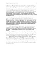
Suppose that the price of a bushel of tomatoes is $9, or P
2
in Figure 2.5. At this price the
quantity demanded by consumers is 20,000 bushels, much less than the quantity offered by

Chapter 2 Competitive Product Markets


12
producers, 90,000. There is a market surplus, or excess supply, of 70,000 bushels. A market
surplus is the amount by which the quantity supplied exceeds the quantity demanded at any
given price. Graphically, an excess quantity supplied occurs at any price above the intersection
of the supply and demand curves.




FIGURE 2.5 Market Surplus
If a price is higher than the intersection of the supply
and demand curves, a market surplus—a greater
quantity supplied, Q
3
, than demanded, Q
1
—results.
Competitive pressure will push the price down to the
equilibrium price P
1
, the price at which the quantity

supplied equals the quantity demanded (Q
2
).





What will happen in this situation? Producers who cannot sell their tomatoes will have to
compete by offering to sell at a lower price, forcing other producers to follow suit. As the
competitive process forces the price down, the quantity consumers are willing to buy will
expand, while the quantity producers are willing to sell will decrease. The result will be a
contraction of the surplus, until it is finally eliminated at a price of $5.50 or P
1
(at the intersection
of the two curves). At that price, producers will be selling all they want to; they will see no
reason to lower prices further. Similarly, consumers will see no reason to pay more; they will be
buying all they want. This point, where the wants of buyers and sellers intersect, is called the
equilibrium price.
• The equilibrium price is the price toward which a competitive market will move,
and at which it will remain once there, everything else held constant. It is the price
at which the market “clears”—that is, at which the quantity demanded by
consumers is matched exactly by the quantity offered by producers. At the
equilibrium price, the quantities desired by buyers and sellers are also equal. This is
the equilibrium quantity.
• The equilibrium quantity is the output (or sales) level toward which the market
will move, and at which it will remain once there, everything else held constant.

Chapter 2 Competitive Product Markets

13
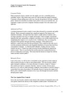
In sum, a surplus emerges when the price asked is above the equilibrium price. It will
be eliminated, through competition among sellers, when the price drops to the equilibrium price.

Market Shortages
Suppose the price asked is below the equilibrium price, as in Figure 2.6. At the relatively low
price of $1, or P
1
, buyers want to purchase 100,000 bushels—substantially more than the
10,000 bushels producers are willing to offer. The result is a market shortage. A market
shortage is the amount by which the quantity demanded exceeds the quantity supplied at any
given price. Graphically, it is the shortfall that occurs any price below the intersection of the
supply and demand curves.
As with a market surplus, competition will correct the discrepancy between buyers’ and
sellers’ plans. Buyers who want tomatoes but are unable to get them at a price of $1 will bid
higher prices, as at an auction. As the price rises, a larger quantity will be supplied because
suppliers will be better able to cover their increasing production costs. At the same time the
quantity demanded will contract as buyers seek substitutes that are now relatively less expensive
compared with tomatoes. At the equilibrium price of $5.50, or P
2
, the market shortage will be
eliminated. Buyers will have no reason to bid prices up further, for they will be getting all the
tomatoes the want at that price. Sellers will have no reason to expand production further; they
will be selling all they want to at that price. The equilibrium price will remain the same until some
force shifts the position of either the supply or the demand curve. If such a shift occurs, the
price will moves toward a new equilibrium at the new intersection of the supply and demand
curves.

FIGURE 2.6 Market Shortages
A price that is below the intersection of the supply
and demand curves will create a shortage—a greater
quantity demanded, Q
3
than supplied Q
1
.
Competitive pressure will push the price up to the
equilibrium price P
2
, the price at which the quantity
supplied equals the quantity demanded.





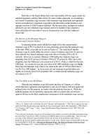
The Effect of Changes in Demand and Supply
Chapter 2 Competitive Product Markets


14
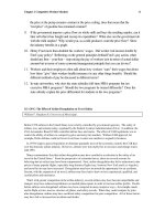
Figure 2.7 shows the effects of shifts in demand and supply on the equilibrium price and
quantity. In panel (a), an increase in demand from D
1
to D
2
raises the equilibrium price from
P

1
to P
2
and quantity from Q
2
to Q
1
. Panel (b) shows the reverse effects of a decrease in
demand.
An increase in supply from S
1
to S
2
-- panel (c) has a different effect. The equilibrium
quantity rises from Q
1
to Q
2
, but the equilibrium price falls from P
2
to P
1
. A decrease in supply
from S
1
to S
2
-- panel (d) -- causes the opposite effect: the equilibrium quantity falls from Q
2
to

Q
1
, and the equilibrium price rises from P
1
to P
2
.




















FIGURE 2.7 The Effects of Changes in Supply and Demand
An increase in demand—panel (a) -- raises both the equilibrium price and the equilibrium
quantity. A decrease in demand -- panel (b) -- has the opposite effect: a decrease in the

equilibrium price and quantity. An increase in supply -- panel (c)—causes the equilibrium
quantity to rise but the equilibrium price to fall. A decrease in supply -- panel (d) -- has the
opposite effect: a rise in the equilibrium price and a fall in the equilibrium quantity.