Tài liệu Ten Principles of Economics - Part 10 ppt

CHAPTER 5 ELASTICITY AND ITS APPLICATION 95
little concern over his health, sailboats might be a necessity with inelastic demand
and doctor visits a luxury with elastic demand.
Availability of Close Substitutes
Goods with close substitutes tend
to have more elastic demand because it is easier for consumers to switch from that
good to others. For example, butter and margarine are easily substitutable. A small
increase in the price of butter, assuming the price of margarine is held fixed, causes
the quantity of butter sold to fall by a large amount. By contrast, because eggs are
a food without a close substitute, the demand for eggs is probably less elastic than
the demand for butter.
Definition of the Market
The elasticity of demand in any market de-
pends on how we draw the boundaries of the market. Narrowly defined markets
tend to have more elastic demand than broadly defined markets, because it is
easier to find close substitutes for narrowly defined goods. For example, food, a
broad category, has a fairly inelastic demand because there are no good substitutes
for food. Ice cream, a more narrow category, has a more elastic demand because it
is easy to substitute other desserts for ice cream. Vanilla ice cream, a very narrow
category, has a very elastic demand because other flavors of ice cream are almost
perfect substitutes for vanilla.
Time Horizon
Goods tend to have more elastic demand over longer time
horizons. When the price of gasoline rises, the quantity of gasoline demanded falls
only slightly in the first few months. Over time, however, people buy more fuel-
efficient cars, switch to public transportation, and move closer to where they work.
Within several years, the quantity of gasoline demanded falls substantially.
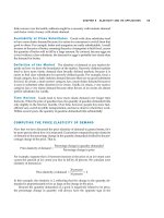
COMPUTING THE PRICE ELASTICITY OF DEMAND
Now that we have discussed the price elasticity of demand in general terms, let’s
be more precise about how it is measured. Economists compute the price elasticity
of demand as the percentage change in the quantity demanded divided by the per-

centage change in the price. That is,
Price elasticity of demand ϭ .
For example, suppose that a 10-percent increase in the price of an ice-cream cone
causes the amount of ice cream you buy to fall by 20 percent. We calculate your
elasticity of demand as
Price elasticity of demand ϭϭ2.
In this example, the elasticity is 2, reflecting that the change in the quantity de-
manded is proportionately twice as large as the change in the price.
Because the quantity demanded of a good is negatively related to its price,
the percentage change in quantity will always have the opposite sign as the
20 percent
10 percent
Percentage change in quantity demanded
Percentage change in price
96 PART TWO SUPPLY AND DEMAND I: HOW MARKETS WORK
percentage change in price. In this example, the percentage change in price is a pos-
itive 10 percent (reflecting an increase), and the percentage change in quantity de-
manded is a negative 20 percent (reflecting a decrease). For this reason, price
elasticities of demand are sometimes reported as negative numbers. In this book
we follow the common practice of dropping the minus sign and reporting all price
elasticities as positive numbers. (Mathematicians call this the absolute value.) With
this convention, a larger price elasticity implies a greater responsiveness of quan-
tity demanded to price.
THE MIDPOINT METHOD: A BETTER WAY TO CALCULATE
PERCENTAGE CHANGES AND ELASTICITIES
If you try calculating the price elasticity of demand between two points on a de-
mand curve, you will quickly notice an annoying problem: The elasticity from
point A to point B seems different from the elasticity from point B to point A. For
example, consider these numbers:
Point A: Price ϭ $4 Quantity ϭ 120

Point B: Price ϭ $6 Quantity ϭ 80
Going from point A to point B, the price rises by 50 percent, and the quantity falls
by 33 percent, indicating that the price elasticity of demand is 33/50, or 0.66.
By contrast, going from point B to point A, the price falls by 33 percent, and the
quantity rises by 50 percent, indicating that the price elasticity of demand is 50/33,
or 1.5.
One way to avoid this problem is to use the midpoint method for calculating
elasticities. Rather than computing a percentage change using the standard way
(by dividing the change by the initial level), the midpoint method computes a
percentage change by dividing the change by the midpoint of the initial and final
levels. For instance, $5 is the midpoint of $4 and $6. Therefore, according to the
midpoint method, a change from $4 to $6 is considered a 40 percent rise, because
(6 Ϫ 4)/5 ϫ 100 ϭ 40. Similarly, a change from $6 to $4 is considered a 40 per-
cent fall.
Because the midpoint method gives the same answer regardless of the direc-
tion of change, it is often used when calculating the price elasticity of demand be-
tween two points. In our example, the midpoint between point A and point B is:
Midpoint: Price ϭ $5 Quantity ϭ 100
According to the midpoint method, when going from point A to point B, the price
rises by 40 percent, and the quantity falls by 40 percent. Similarly, when going
from point B to point A, the price falls by 40 percent, and the quantity rises by
40 percent. In both directions, the price elasticity of demand equals 1.
We can express the midpoint method with the following formula for the price
elasticity of demand between two points, denoted (Q
1
, P
1
) and (Q
2
, P

2
):
Price elasticity of demand ϭ .
(Q
2
Ϫ Q
1
)/[(Q
2
ϩ Q
1
)/2]
(P
2
Ϫ P
1
)/[(P
2
ϩ P
1
)/2]
(a) Perfectly Inelastic Demand: Elasticity Equals 0
$5
4
Demand
Quantity
1000
(b) Inelastic Demand: Elasticity Is Less Than 1
$5
4

Quantity
1000 90
Demand
(c) Unit Elastic Demand: Elasticity Equals 1
$5
4
Demand
Quantity
1000
Price
80
1. An
increase
in price . . .
2. . . . leaves the quantity demanded unchanged.
2. . . . leads to a 22% decrease in quantity demanded.
1. A 22%
increase
in price . . .
Price Price
2. . . . leads to an 11% decrease in quantity demanded.
1. A 22%
increase
in price . . .
(d) Elastic Demand: Elasticity Is Greater Than 1
$5
4
Demand
Quantity
1000

Price
50
(e) Perfectly Elastic Demand: Elasticity Equals Infinity
$4
Quantity
0
Price
Demand
1. A 22%
increase
in price . . .
2. At exactly $4,
consumers will
buy any quantity.
1. At any price
above $4, quantity
demanded is zero.
2. . . . leads to a 67% decrease in quantity demanded.
3. At a price below $4,
quantity demanded is infinite.
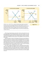
Figure 5-1
T
HE
P
RICE
E
LASTICITY OF
D
EMAND
. The price elasticity of demand determines whether

the demand curve is steep or flat. Note that all percentage changes are calculated using
the midpoint method.
98 PART TWO SUPPLY AND DEMAND I: HOW MARKETS WORK
The numerator is the percentage change in quantity computed using the midpoint
method, and the denominator is the percentage change in price computed using
the midpoint method. If you ever need to calculate elasticities, you should use this
formula.
Throughout this book, however, we only rarely need to perform such calcula-
tions. For our purposes, what elasticity represents—the responsiveness of quantity
demanded to price—is more important than how it is calculated.
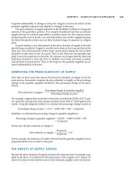
THE VARIETY OF DEMAND CURVES
Economists classify demand curves according to their elasticity. Demand is elastic
when the elasticity is greater than 1, so that quantity moves proportionately more
than the price. Demand is inelastic when the elasticity is less than 1, so that quan-
tity moves proportionately less than the price. If the elasticity is exactly 1, so that
quantity moves the same amount proportionately as price, demand is said to have
unit elasticity.
Because the price elasticity of demand measures how much quantity de-
manded responds to changes in the price, it is closely related to the slope of the de-
mand curve. The following rule of thumb is a useful guide: The flatter is the
demand curve that passes through a given point, the greater is the price elasticity
of demand. The steeper is the demand curve that passes through a given point, the
smaller is the price elasticity of demand.
Figure 5-1 shows five cases. In the extreme case of a zero elasticity, demand is
perfectly inelastic, and the demand curve is vertical. In this case, regardless of the
price, the quantity demanded stays the same. As the elasticity rises, the demand
curve gets flatter and flatter. At the opposite extreme, demand is perfectly elastic.
This occurs as the price elasticity of demand approaches infinity and the demand
curve becomes horizontal, reflecting the fact that very small changes in the price
lead to huge changes in the quantity demanded.

Finally, if you have trouble keeping straight the terms elastic and inelastic,
here’s a memory trick for you: Inelastic curves, such as in panel (a) of Figure 5-1,
look like the letter I. Elastic curves, as in panel (e), look like the letter E. This is not
a deep insight, but it might help on your next exam.
TOTAL REVENUE AND THE PRICE ELASTICITY OF DEMAND
When studying changes in supply or demand in a market, one variable we often
want to study is total revenue, the amount paid by buyers and received by sellers
of the good. In any market, total revenue is P ϫ Q, the price of the good times the
quantity of the good sold. We can show total revenue graphically, as in Figure 5-2.
The height of the box under the demand curve is P, and the width is Q. The area
of this box, P ϫ Q, equals the total revenue in this market. In Figure 5-2, where
P ϭ $4 and Q ϭ 100, total revenue is $4 ϫ 100, or $400.
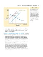
How does total revenue change as one moves along the demand curve? The
answer depends on the price elasticity of demand. If demand is inelastic, as in Fig-
ure 5-3, then an increase in the price causes an increase in total revenue. Here an
increase in price from $1 to $3 causes the quantity demanded to fall only from 100
total revenue
the amount paid by buyers and
received by sellers of a good,
computed as the price of the good
times the quantity sold
CHAPTER 5 ELASTICITY AND ITS APPLICATION 99
$4
Demand
Quantity
Q
P
0
Price
P

ϫ

Q

ϭ
$400
(revenue)
100
Figure 5-2
T
OTAL
R
EVENUE
. The total
amount paid by buyers, and
received as revenue by sellers,
equals the area of the box under
the demand curve, P ϫ Q. Here,
at a price of $4, the quantity
demanded is 100, and total
revenue is $400.
$1
Demand
Quantity
0
Price
Revenue
ϭ
$100

100
$3
Quantity
0
Price
80
Revenue
ϭ
$240
Demand
Figure 5-3
H
OW
T
OTAL
R
EVENUE
C
HANGES
W
HEN
P
RICE
C
HANGES
: I
NELASTIC
D
EMAND
. With an

inelastic demand curve, an increase in the price leads to a decrease in quantity demanded
that is proportionately smaller. Therefore, total revenue (the product of price and quantity)
increases. Here, an increase in the price from $1 to $3 causes the quantity demanded to fall
from 100 to 80, and total revenue rises from $100 to $240.