Tài liệu Ten Principles of Economics - Part 11 pdf

CHAPTER 5 ELASTICITY AND ITS APPLICATION 105
responds substantially to changes in the price. Supply is said to be inelastic if the
quantity supplied responds only slightly to changes in the price.
The price elasticity of supply depends on the flexibility of sellers to change the
amount of the good they produce. For example, beachfront land has an inelastic
supply because it is almost impossible to produce more of it. By contrast, manu-
factured goods, such as books, cars, and televisions, have elastic supplies because
the firms that produce them can run their factories longer in response to a higher
price.
In most markets, a key determinant of the price elasticity of supply is the time
period being considered. Supply is usually more elastic in the long run than in the
short run. Over short periods of time, firms cannot easily change the size of their
factories to make more or less of a good. Thus, in the short run, the quantity sup-
plied is not very responsive to the price. By contrast, over longer periods, firms can
build new factories or close old ones. In addition, new firms can enter a market,
and old firms can shut down. Thus, in the long run, the quantity supplied can re-
spond substantially to the price.
COMPUTING THE PRICE ELASTICITY OF SUPPLY
Now that we have some idea about what the price elasticity of supply is, let’s be
more precise. Economists compute the price elasticity of supply as the percentage
change in the quantity supplied divided by the percentage change in the price.
That is,
Price elasticity of supply ϭ .
For example, suppose that an increase in the price of milk from $2.85 to $3.15 a gal-
lon raises the amount that dairy farmers produce from 9,000 to 11,000 gallons per
month. Using the midpoint method, we calculate the percentage change in price as
Percentage change in price ϭ (3.15 Ϫ 2.85)/3.00 ϫ 100 ϭ 10 percent.
Similarly, we calculate the percentage change in quantity supplied as
Percentage change in quantity supplied ϭ (11,000 Ϫ 9,000)/10,000 ϫ 100
ϭ 20 percent.
In this case, the price elasticity of supply is

Price elasticity of supply ϭϭ2.0.
In this example, the elasticity of 2 reflects the fact that the quantity supplied moves
proportionately twice as much as the price.
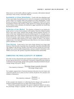
THE VARIETY OF SUPPLY CURVES
Because the price elasticity of supply measures the responsiveness of quantity sup-
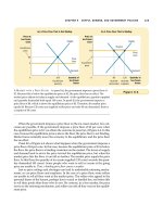
plied to the price, it is reflected in the appearance of the supply curve. Figure 5-6
shows five cases. In the extreme case of a zero elasticity, supply is perfectly inelastic,
20 percent
10 percent
Percentage change in quantity supplied
Percentage change in price
100 110
100 125
(a) Perfectly Inelastic Supply: Elasticity Equals 0
$5
4
Supply
Quantity
1000
(b) Inelastic Supply: Elasticity Is Less Than 1
$5
4
Quantity
0
(c) Unit Elastic Supply: Elasticity Equals 1
$5
4
Quantity
0
Price

1. An
increase
in price . . .
2. . . . leaves the quantity supplied unchanged.
2. . . . leads to a 22% increase in quantity supplied.
1. A 22%
increase
in price . . .
Price Price
2. . . . leads to a 10% increase in quantity supplied.
1. A 22%
increase
in price . . .
(d) Elastic Supply: Elasticity Is Greater Than 1
$5
4
Quantity
0
Price
(e) Perfectly Elastic Supply: Elasticity Equals Infinity
$4
Quantity
0
Price
Supply
1. A 22%
increase
in price . . .
2. At exactly $4,
producers will

supply any quantity.
1. At any price
above $4, quantity
supplied is infinite.
2. . . . leads to a 67% increase in quantity supplied.
3. At a price below $4,
quantity supplied is zero.
Supply
Supply
100 200
Supply
Figure 5-6
T
HE
P
RICE
E
LASTICITY OF
S
UPPLY
. The price elasticity of supply determines whether the
supply curve is steep or flat. Note that all percentage changes are calculated using the
midpoint method.
CHAPTER 5 ELASTICITY AND ITS APPLICATION 107
and the supply curve is vertical. In this case, the quantity supplied is the same re-
gardless of the price. As the elasticity rises, the supply curve gets flatter, which
shows that the quantity supplied responds more to changes in the price. At the op-
posite extreme, supply is perfectly elastic. This occurs as the price elasticity of sup-
ply approaches infinity and the supply curve becomes horizontal, meaning that
very small changes in the price lead to very large changes in the quantity supplied.

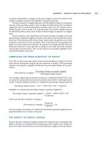
In some markets, the elasticity of supply is not constant but varies over the
supply curve. Figure 5-7 shows a typical case for an industry in which firms have
factories with a limited capacity for production. For low levels of quantity sup-
plied, the elasticity of supply is high, indicating that firms respond substantially to
changes in the price. In this region, firms have capacity for production that is not
being used, such as plants and equipment sitting idle for all or part of the day.
Small increases in price make it profitable for firms to begin using this idle capac-
ity. As the quantity supplied rises, firms begin to reach capacity. Once capacity is
fully used, increasing production further requires the construction of new plants.
To induce firms to incur this extra expense, the price must rise substantially, so
supply becomes less elastic.
Figure 5-7 presents a numerical example of this phenomenon. When the price
rises from $3 to $4 (a 29 percent increase, according to the midpoint method), the
quantity supplied rises from 100 to 200 (a 67 percent increase). Because quantity
supplied moves proportionately more than the price, the supply curve has elastic-
ity greater than 1. By contrast, when the price rises from $12 to $15 (a 22 percent in-
crease), the quantity supplied rises from 500 to 525 (a 5 percent increase). In this
case, quantity supplied moves proportionately less than the price, so the elasticity
is less than 1.
QUICK QUIZ: Define the price elasticity of supply. ◆ Explain why the
the price elasticity of supply might be different in the long run than in the
short run.
$15
12
3
Quantity
100 200 5000
Price
525
Elasticity is small

(less than 1).
Elasticity is large
(greater than 1).
4
Figure 5-7
H
OW THE
P
RICE
E
LASTICITY OF
S
UPPLY
C
AN
V
ARY
. Because
firms often have a maximum
capacity for production, the
elasticity of supply may be very
high at low levels of quantity
supplied and very low at high
levels of quantity supplied. Here,
an increase in price from $3 to $4
increases the quantity supplied
from 100 to 200. Because the
increase in quantity supplied of
67 percent is larger than the
increase in price of 29 percent, the

supply curve is elastic in this
range. By contrast, when the
price rises from $12 to $15, the
quantity supplied rises only from
500 to 525. Because the increase in
quantity supplied of 5 percent is
smaller than the increase in price
of 22 percent, the supply curve is
inelastic in this range.
108 PART TWO SUPPLY AND DEMAND I: HOW MARKETS WORK
THREE APPLICATIONS OF SUPPLY,
DEMAND, AND ELASTICITY
Can good news for farming be bad news for farmers? Why did the Organization of
Petroleum Exporting Countries (OPEC) fail to keep the price of oil high? Does
drug interdiction increase or decrease drug-related crime? At first, these questions
might seem to have little in common. Yet all three questions are about markets,
and all markets are subject to the forces of supply and demand. Here we apply the
versatile tools of supply, demand, and elasticity to answer these seemingly com-
plex questions.
CAN GOOD NEWS FOR FARMING BE
BAD NEWS FOR FARMERS?
Let’s now return to the question posed at the beginning of this chapter: What hap-
pens to wheat farmers and the market for wheat when university agronomists dis-
cover a new wheat hybrid that is more productive than existing varieties? Recall
from Chapter 4 that we answer such questions in three steps. First, we examine
whether the supply curve or demand curve shifts. Second, we consider which di-
rection the curve shifts. Third, we use the supply-and-demand diagram to see how
the market equilibrium changes.
In this case, the discovery of the new hybrid affects the supply curve. Because
the hybrid increases the amount of wheat that can be produced on each acre of

land, farmers are now willing to supply more wheat at any given price. In other
words, the supply curve shifts to the right. The demand curve remains the same
because consumers’ desire to buy wheat products at any given price is not affected
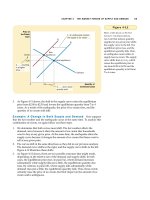
by the introduction of a new hybrid. Figure 5-8 shows an example of such a
change. When the supply curve shifts from S
1
to S
2
, the quantity of wheat sold in-
creases from 100 to 110, and the price of wheat falls from $3 to $2.
But does this discovery make farmers better off? As a first cut to answering
this question, consider what happens to the total revenue received by farmers.
Farmers’ total revenue is P ϫ Q, the price of the wheat times the quantity sold. The
discovery affects farmers in two conflicting ways. The hybrid allows farmers to
produce more wheat (Q rises), but now each bushel of wheat sells for less (P falls).
Whether total revenue rises or falls depends on the elasticity of demand. In
practice, the demand for basic foodstuffs such as wheat is usually inelastic, for
these items are relatively inexpensive and have few good substitutes. When the
demand curve is inelastic, as it is in Figure 5-8, a decrease in price causes total rev-
enue to fall. You can see this in the figure: The price of wheat falls substantially,
whereas the quantity of wheat sold rises only slightly. Total revenue falls from
$300 to $220. Thus, the discovery of the new hybrid lowers the total revenue that
farmers receive for the sale of their crops.
If farmers are made worse off by the discovery of this new hybrid, why do
they adopt it? The answer to this question goes to the heart of how competitive
markets work. Because each farmer is a small part of the market for wheat, he or
she takes the price of wheat as given. For any given price of wheat, it is better to
CHAPTER 5 ELASTICITY AND ITS APPLICATION 109
use the new hybrid in order to produce and sell more wheat. Yet when all farmers
do this, the supply of wheat rises, the price falls, and farmers are worse off.

Although this example may at first seem only hypothetical, in fact it helps to
explain a major change in the U.S. economy over the past century. Two hundred
years ago, most Americans lived on farms. Knowledge about farm methods was
sufficiently primitive that most of us had to be farmers to produce enough food.
Yet, over time, advances in farm technology increased the amount of food that
each farmer could produce. This increase in food supply, together with inelastic
food demand, caused farm revenues to fall, which in turn encouraged people to
leave farming.
A few numbers show the magnitude of this historic change. As recently as
1950, there were 10 million people working on farms in the United States, repre-
senting 17 percent of the labor force. In 1998, fewer than 3 million people worked
on farms, or 2 percent of the labor force. This change coincided with tremendous
advances in farm productivity: Despite the 70 percent drop in the number of farm-
ers, U.S. farms produced more than twice the output of crops and livestock in 1998
as they did in 1950.
This analysis of the market for farm products also helps to explain a seeming
paradox of public policy: Certain farm programs try to help farmers by inducing
them not to plant crops on all of their land. Why do these programs do this? Their
purpose is to reduce the supply of farm products and thereby raise prices. With in-
elastic demand for their products, farmers as a group receive greater total revenue
if they supply a smaller crop to the market. No single farmer would choose to
leave his land fallow on his own because each takes the market price as given. But
if all farmers do so together, each of them can be better off.
$3
2
Quantity of Wheat
1000
Price of
Wheat
1. When demand is inelastic,

an increase in supply . . .
3. . . . and a proportionately smaller
increase in quantity sold. As a result,
revenue falls from $300 to $220.
110
Demand
S
1
S
2
2. . . . leads
to a large
fall in
price . . .
Figure 5-8
A
N
I
NCREASE IN
S
UPPLY IN THE
M
ARKET FOR
W
HEAT
. When an
advance in farm technology
increases the supply of wheat
from S
1

to S
2
, the price of wheat
falls. Because the demand for
wheat is inelastic, the increase in
the quantity sold from 100 to 110
is proportionately smaller than
the decrease in the price from
$3 to $2. As a result, farmers’
total revenue falls from $300
($3 ϫ 100) to $220 ($2 ϫ 110).