Tài liệu Ten Principles of Economics - Part 56 pdf

CHAPTER 25 SAVING, INVESTMENT, AND THE FINANCIAL SYSTEM 569
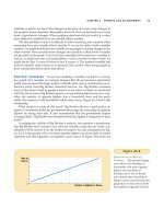
billion to $1,600 billion. That is, the shift in the supply curve moves the market
equilibrium along the demand curve. With a lower cost of borrowing, households
and firms are motivated to borrow more to finance greater investment. Thus, if a
change in the tax laws encouraged greater saving, the result would be lower interest rates
and greater investment.
Although this analysis of the effects of increased saving is widely accepted
among economists, there is less consensus about what kinds of tax changes should
be enacted. Many economists endorse tax reform aimed at increasing saving in or-
der to stimulate investment and growth. Yet others are skeptical that these tax
changes would have much effect on national saving. These skeptics also doubt the
equity of the proposed reforms. They argue that, in many cases, the benefits of the
tax changes would accrue primarily to the wealthy, who are least in need of tax re-
lief. We examine this debate more fully in the final chapter of this book.
POLICY 2: TAXES AND INVESTMENT
Suppose that Congress passed a law giving a tax reduction to any firm building a
new factory. In essence, this is what Congress does when it institutes an investment
tax credit, which it does from time to time. Let’s consider the effect of such a law on
the market for loanable funds, as illustrated in Figure 25-3.
First, would the law affect supply or demand? Because the tax credit would
reward firms that borrow and invest in new capital, it would alter investment at
any given interest rate and, thereby, change the demand for loanable funds. By
contrast, because the tax credit would not affect the amount that households save
at any given interest rate, it would not affect the supply of loanable funds.
Loanable Funds
(in billions of dollars)
0
Interest
Rate
4%
5%

Supply,
S
1
S
2
$1,200 $1,600
2. ...which
reduces the
equilibrium
interest rate...
3. ...and raises the equilibrium
quantity of loanable funds.
Demand
1. Tax incentives for
saving increase the
supply of loanable
funds...
Figure 25-2
A
N
I
NCREASE IN THE
S
UPPLYOF
L
OANABLE
F
UNDS
. A change
in the tax laws to encourage

Americans to save more would
shift the supply of loanable funds
to the right from S
1
to S
2
. As a
result, the equilibrium interest
rate would fall, and the lower
interest rate would stimulate
investment. Here the equilibrium
interest rate falls from 5 percent
to 4 percent, and the equilibrium
quantity of loanable funds saved
and invested rises from $1,200
billion to $1,600 billion.
570 PART NINE THE REAL ECONOMY IN THE LONG RUN
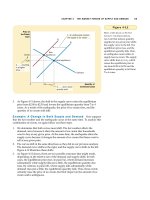
Second, which way would the demand curve shift? Because firms would have
an incentive to increase investment at any interest rate, the quantity of loanable
funds demanded would be higher at any given interest rate. Thus, the demand
curve for loanable funds would move to the right, as shown by the shift from D
1
to
D
2
in the figure.
Third, consider how the equilibrium would change. In Figure 25-3, the in-
creased demand for loanable funds raises the interest rate from 5 percent to 6 per-
cent, and the higher interest rate in turn increases the quantity of loanable funds
supplied from $1,200 billion to $1,400 billion, as households respond by increasing

the amount they save. This change in household behavior is represented here as a
movement along the supply curve. Thus, if a change in the tax laws encouraged
greater investment, the result would be higher interest rates and greater saving.
POLICY 3:
GOVERNMENT BUDGET DEFICITS AND SURPLUSES
Throughout the 1980s and 1990s, one of the most pressing policy issues was the
size of the government budget deficit. Recall that a budget deficit is an excess of
government spending over tax revenue. Governments finance budget deficits by
borrowing in the bond market, and the accumulation of past government borrow-
ing is called the government debt. In the 1980s and 1990s, the U.S. federal govern-
ment ran large budget deficits, resulting in a rapidly growing government debt. As
a result, much public debate centered on the effects of these deficits both on the al-
location of the economy’s scarce resources and on long-term economic growth.
Loanable Funds
(in billions of dollars)
0
Interest
Rate
5%
6%
$1,200 $1,400
1. An investment
tax credit
increases the
demand for
loanable funds...
2. ...which
raises the
equilibrium
interest rate...

3. ...and raises the equilibrium
quantity of loanable funds.
Supply
Demand,
D
1

D
2
Figure 25-3
A
N
I
NCREASE IN THE
D
EMAND
FOR
L
OANABLE
F
UNDS
. If the
passage of an investment tax
credit encouraged U.S. firms
to invest more, the demand for
loanable funds would increase.
As a result, the equilibrium
interest rate would rise, and
the higher interest rate would
stimulate saving. Here, when the

demand curve shifts from D
1
to
D
2
, the equilibrium interest rate
rises from 5 percent to 6 percent,
and the equilibrium quantity
of loanable funds saved and
invested rises from $1,200 billion
to $1,400 billion.
CHAPTER 25 SAVING, INVESTMENT, AND THE FINANCIAL SYSTEM 571
We can analyze the effects of a budget deficit by following our three steps in
the market for loanable funds, which is illustrated in Figure 25-4. First, which
curve shifts when the budget deficit rises? Recall that national saving—the source
of the supply of loanable funds—is composed of private saving and public saving.
A change in the government budget deficit represents a change in public saving
and, thereby, in the supply of loanable funds. Because the budget deficit does not
influence the amount that households and firms want to borrow to finance invest-
ment at any given interest rate, it does not alter the demand for loanable funds.
Second, which way does the supply curve shift? When the government runs a
budget deficit, public saving is negative, and this reduces national saving. In other
words, when the government borrows to finance its budget deficit, it reduces the
supply of loanable funds available to finance investment by households and firms.
Thus, a budget deficit shifts the supply curve for loanable funds to the left from
S
1
to S
2
, as shown in Figure 25-4.

Third, we can compare the old and new equilibria. In the figure, when the
budget deficit reduces the supply of loanable funds, the interest rate rises from
5 percent to 6 percent. This higher interest rate then alters the behavior of the
households and firms that participate in the loan market. In particular, many
demanders of loanable funds are discouraged by the higher interest rate. Fewer
families buy new homes, and fewer firms choose to build new factories. The fall in
investment because of government borrowing is called crowding out and is repre-
sented in the figure by the movement along the demand curve from a quantity of
$1,200 billion in loanable funds to a quantity of $800 billion. That is, when the gov-
ernment borrows to finance its budget deficit, it crowds out private borrowers
who are trying to finance investment.
Loanable Funds
(in billions of dollars)
0
Interest
Rate
$800 $1,200
3. ...and reduces the equilibrium
quantity of loanable funds.
S
2
2. ...which
raises the
equilibrium
interest rate...
Supply,
S
1
Demand
5%

6%
1. A budget deficit
decreases the
supply of loanable
funds...
Figure 25-4
T
HE
E
FFECT OF A
G
OVERNMENT
B
UDGET
D
EFICIT
. When the
government spends more than
it receives in tax revenue, the
resulting budget deficit lowers
national saving. The supply of
loanable funds decreases, and
the equilibrium interest rate rises.
Thus, when the government
borrows to finance its budget
deficit, it crowds out households
and firms who otherwise would
borrow to finance investment.
Here, when the supply shifts
from S

1
to S
2
, the equilibrium
interest rate rises from 5 percent
to 6 percent, and the equilibrium
quantity of loanable funds saved
and invested falls from $1,200
billion to $800 billion.
crowding out
a decrease in investment that results
from government borrowing
572 PART NINE THE REAL ECONOMY IN THE LONG RUN
CASE STUDY
THE DEBATE OVER THE BUDGET SURPLUS
Our analysis shows why, other things being the same, budget surpluses are bet-
ter for economic growth than budget deficits. Making economic policy, how-
ever, is not as simple as this observation may make it sound. A good example
occurred in the late 1990s, when the U.S. government found itself with a budget
surplus, and much debate centered on what to do with it.
Many policymakers favored leaving the budget surplus alone, rather than
dissipating it with a spending increase or tax cut. They based their conclusion
on the analysis we have just seen: Using the surplus to retire some of the gov-
ernment debt would stimulate private investment and economic growth.
Other policymakers took a different view. Some thought the surplus should
be used to increase government spending on infrastructure and education be-
cause, they argued, the return to these public investments is greater than the
typical return to private investment. Some thought taxes should be cut, arguing
that lower tax rates would distort decisionmaking less and lead to a more effi-
cient allocation of resources; they also cautioned that without such a tax cut,

Thus, the most basic lesson about budget deficits follows directly from their ef-
fects on the supply and demand for loanable funds: When the government reduces
national saving by running a budget deficit, the interest rate rises, and investment falls.
Because investment is important for long-run economic growth, government bud-
get deficits reduce the economy’s growth rate.
Government budget surpluses work just the opposite as budget deficits. When
government collects more in tax revenue than it spends, its saves the difference by
retiring some of the outstanding government debt. This budget surplus, or public
saving, contributes to national saving. Thus, a budget surplus increases the supply of
loanable funds, reduces the interest rate, and stimulates investment. Higher investment,
in turn, means greater capital accumulation and more rapid economic growth.
“Our debt-reduction
plan is simple, but it
will require a great
deal of money.”
CHAPTER 25 SAVING, INVESTMENT, AND THE FINANCIAL SYSTEM 573
Congress would be tempted to spend the surplus on “pork barrel” projects of
dubious value.
As this book was going to press, the debate over the budget surplus was
still raging. There is room for reasonable people to disagree. The right policy
depends on how valuable you view private investment, how valuable you view
public investment, how distortionary you view taxation, and how reliable you
view the political process.
CASE STUDY
THE HISTORY OF U.S. GOVERNMENT DEBT
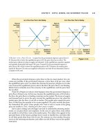
How indebted is the U.S. government? The answer to this question varies sub-
stantially over time. Figure 25-5 shows the debt of the U.S. federal government
expressed as a percentage of U.S. GDP. It shows that the government debt has
fluctuated from zero in 1836 to 107 percent of GDP in 1945. In recent years, gov-
ernment debt has been about 50 percent of GDP.

The behavior of the debt–GDP ratio is one gauge of what’s happening with
the government’s finances. Because GDP is a rough measure of the govern-
ment’s tax base, a declining debt–GDP ratio indicates that the government in-
debtedness is shrinking relative to its ability to raise tax revenue. This suggests
that the government is, in some sense, living within its means. By contrast, a ris-
ing debt–GDP ratio means that the government indebtedness is increasing rela-
tive to its ability to raise tax revenue. It is often interpreted as meaning that
fiscal policy—government spending and taxes—cannot be sustained forever at
current levels.
Throughout history, the primary cause of fluctuations in government
debt is war. When wars occur, government spending on national defense rises
Percent
of GDP
1790 1810 1830 1850 1870 1890 1910 1930 1950 1970 1990
Revolutionary
War
2010
Civil
War
World War I
World War II
0
20
40
60
80
100
120
Figure 25-5
T

HE
U.S. G
OVERNMENT
D
EBT
.
The debt of the U.S. federal
government, expressed here as
a percentage of GDP, has varied
substantially throughout history.
It reached its highest level after
the large expenditures of World
War II, but then declined through-
out the 1950s and 1960s. It began
rising again in the early 1980s
when Ronald Reagan’s tax cuts
were not accompanied by similar
cuts in government spending.
It then stabilized and even
declined slightly in the late 1990s.
Source: U.S. Department of Treasury; U.S.
Department of Commerce; and T. S. Berry,
“Production and Population since 1789,”
Bostwick Paper No. 6, Richmond, 1988.