Tài liệu Ten Principles of Economics - Part 62 ppt

CHAPTER 28 MONEY GROWTH AND INFLATION 631
checking accounts. That is, a higher price level (a lower value of money) increases
the quantity of money demanded.
What ensures that the quantity of money the Fed supplies balances the quan-
tity of money people demand? The answer, it turns out, depends on the time hori-
zon being considered. Later in this book we will examine the short-run answer,
and we will see that interest rates play a key role. In the long run, however, the an-
swer is different and much simpler. In the long run, the overall level of prices adjusts
to the level at which the demand for money equals the supply. If the price level is above
the equilibrium level, people will want to hold more money than the Fed has cre-
ated, so the price level must fall to balance supply and demand. If the price level is
below the equilibrium level, people will want to hold less money than the Fed has
created, and the price level must rise to balance supply and demand. At the equi-
librium price level, the quantity of money that people want to hold exactly bal-
ances the quantity of money supplied by the Fed.
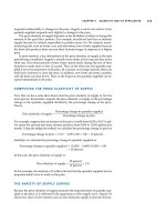
Figure 28-1 illustrates these ideas. The horizontal axis of this graph shows the
quantity of money. The left-hand vertical axis shows the value of money, 1/P, and
the right-hand vertical axis shows the price level, P. Notice that the price-level axis
on the right is inverted: A low price level is shown near the top of this axis, and a
high price level is shown near the bottom. This inverted axis illustrates that when
the value of money is high (as shown near the top of the left axis), the price level is
low (as shown near the top of the right axis).
The two curves in this figure are the supply and demand curves for money.
The supply curve is vertical because the Fed has fixed the quantity of money avail-
able. The demand curve for money is downward sloping, indicating that when the
value of money is low (and the price level is high), people demand a larger quan-
tity of it to buy goods and services. At the equilibrium, shown in the figure as
point A, the quantity of money demanded balances the quantity of money sup-
plied. This equilibrium of money supply and money demand determines the value
of money and the price level.
Quantity fixed

by the Fed
Quantity of
Money
Value of
Money,
1/
P
Price
Level,
P
A
Money supply
0
1
(Low)
(High)
(High)
(Low)
1
/
2
1
/
4
3
/
4
1
1.33
2

4
Equilibrium
value of
money
Equilibrium
price level
Money
demand
Figure 28-1
H
OW THE
S
UPPLY AND
D
EMAND
FOR
M
ONEY
D
ETERMINE THE
E
QUILIBRIUM
P
RICE
L
EVEL
.
The horizontal axis shows the
quantity of money. The left
vertical axis shows the value of

money, and the right vertical axis
shows the price level. The supply
curve for money is vertical
because the quantity of money
supplied is fixed by the Fed.
The demand curve for money
is downward sloping because
people want to hold a larger
quantity of money when
each dollar buys less. At the
equilibrium, point A, the value
of money (on the left axis) and
the price level (on the right
axis) have adjusted to bring the
quantity of money supplied
and the quantity of money
demanded into balance.
632 PART TEN MONEY AND PRICES IN THE LONG RUN
THE EFFECTS OF A MONETARY INJECTION
Let’s now consider the effects of a change in monetary policy. To do so, imagine
that the economy is in equilibrium and then, suddenly, the Fed doubles the supply
of money by printing some dollar bills and dropping them around the country
from helicopters. (Or, less dramatically and more realistically, the Fed could inject
money into the economy by buying some government bonds from the public in
open-market operations.) What happens after such a monetary injection? How
does the new equilibrium compare to the old one?
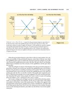
Figure 28-2 shows what happens. The monetary injection shifts the supply
curve to the right from MS
1
to MS

2
, and the equilibrium moves from point A to
point B. As a result, the value of money (shown on the left axis) decreases from 1/2
to 1/4, and the equilibrium price level (shown on the right axis) increases from
2 to 4. In other words, when an increase in the money supply makes dollars more
plentiful, the result is an increase in the price level that makes each dollar less
valuable.
This explanation of how the price level is determined and why it might change
over time is called the quantity theory of money. According to the quantity theory,
the quantity of money available in the economy determines the value of money,
and growth in the quantity of money is the primary cause of inflation. As econo-
mist Milton Friedman once put it, “Inflation is always and everywhere a monetary
phenomenon.”
A BRIEF LOOK AT THE ADJUSTMENT PROCESS
So far we have compared the old equilibrium and the new equilibrium after an in-
jection of money. How does the economy get from the old to the new equilibrium?
Quantity of
Money
Value of
Money,
1/
P
Price
Level,
P
A
B
Money
demand
0

1
(Low)
(High)
(High)
(Low)
1
/
2
1
/
4
3
/
4
1
1.33
2
4
M
1
MS
1
M
2
MS
2
2. …decreases
the value of
money…
3. …and

increases
the price
level.
1. An increase
in the money
supply...
Figure 28-2
A
N
I
NCREASE IN THE
M
ONEY
S
UPPLY
. When the Fed
increases the supply of money,
the money supply curve shifts
from MS
1
to MS
2
. The value of
money (on the left axis) and the
price level (on the right axis)
adjust to bring supply and
demand back into balance. The
equilibrium moves from point
A to point B. Thus, when an
increase in the money supply

makes dollars more plentiful, the
price level increases, making each
dollar less valuable.
quantity theory of money
a theory asserting that the quantity
of money available determines the
price level and that the growth rate
in the quantity of money available
determines the inflation rate
CHAPTER 28 MONEY GROWTH AND INFLATION 633
A complete answer to this question requires an understanding of short-run
fluctuations in the economy, which we examine later in this book. Yet, even now, it
is instructive to consider briefly the adjustment process that occurs after a change
in money supply.
The immediate effect of a monetary injection is to create an excess supply
of money. Before the injection, the economy was in equilibrium (point A in Fig-
ure 28-2). At the prevailing price level, people had exactly as much money as they
wanted. But after the helicopters drop the new money and people pick it up off the
streets, people have more dollars in their wallets than they want. At the prevailing
price level, the quantity of money supplied now exceeds the quantity demanded.
People try to get rid of this excess supply of money in various ways. They
might buy goods and services with their excess holdings of money. Or they might
use this excess money to make loans to others by buying bonds or by depositing
the money in a bank savings account. These loans allow other people to buy goods
and services. In either case, the injection of money increases the demand for
goods and services.
The economy’s ability to supply goods and services, however, has not
changed. As we saw in Chapter 24, the economy’s production is determined by the
available labor, physical capital, human capital, natural resources, and techno-
logical knowledge. None of these is altered by the injection of money.

Thus, the greater demand for goods and services causes the prices of goods
and services to increase. The increase in the price level, in turn, increases the quan-
tity of money demanded because people are using more dollars for every transac-
tion. Eventually, the economy reaches a new equilibrium (point B in Figure 28-2) at
which the quantity of money demanded again equals the quantity of money sup-
plied. In this way, the overall price level for goods and services adjusts to bring
money supply and money demand into balance.
THE CLASSICAL DICHOTOMY AND MONETARY NEUTRALITY
We have seen how changes in the money supply lead to changes in the average
level of prices of goods and services. How do these monetary changes affect other
important macroeconomic variables, such as production, employment, real wages,
and real interest rates? This question has long intrigued economists. Indeed, the
great philosopher David Hume wrote about it in the eighteenth century. The an-
swer we give today owes much to Hume’s analysis.
Hume and his contemporaries suggested that all economic variables should be
divided into two groups. The first group consists of nominal variables—variables
measured in monetary units. The second group consists of real variables—vari-
ables measured in physical units. For example, the income of corn farmers is a
nominal variable because it is measured in dollars, whereas the quantity of corn
they produce is a real variable because it is measured in bushels. Similarly, nomi-
nal GDP is a nominal variable because it measures the dollar value of the econ-
omy’s output of goods and services, while real GDP is a real variable because it
measures the total quantity of goods and services produced. This separation of
variables into these groups is now called the classical dichotomy. (A dichotomy is a
division into two groups, and classical refers to the earlier economic thinkers.)
Application of the classical dichotomy is somewhat tricky when we turn
to prices. Prices in the economy are normally quoted in terms of money and,
nominal variables
variables measured in
monetary units

real variables
variables measured in physical units
classical dichotomy
the theoretical separation of nominal
and real variables
634 PART TEN MONEY AND PRICES IN THE LONG RUN
therefore, are nominal variables. For instance, when we say that the price of corn
is $2 a bushel or that the price of wheat is $1 a bushel, both prices are nominal vari-
ables. But what about a relative price—the price of one thing compared to another?
In our example, we could say that the price of a bushel of corn is two bushels of
wheat. Notice that this relative price is no longer measured in terms of money.
When comparing the prices of any two goods, the dollar signs cancel, and the re-
sulting number is measured in physical units. The lesson is that dollar prices are
nominal variables, whereas relative prices are real variables.
This lesson has several important applications. For instance, the real wage (the
dollar wage adjusted for inflation) is a real variable because it measures the rate at
which the economy exchanges goods and services for each unit of labor. Similarly,
the real interest rate (the nominal interest rate adjusted for inflation) is a real vari-
able because it measures the rate at which the economy exchanges goods and ser-
vices produced today for goods and services produced in the future.
Why bother separating variables into these two groups? Hume suggested that
the classical dichotomy is useful in analyzing the economy because different forces
influence real and nominal variables. In particular, he argued, nominal variables
are heavily influenced by developments in the economy’s monetary system,
whereas the monetary system is largely irrelevant for understanding the determi-
nants of important real variables.
Notice that Hume’s idea was implicit in our earlier discussions of the real
economy in the long run. In previous chapters, we examined how real GDP, sav-
ing, investment, real interest rates, and unemployment are determined without
any mention of the existence of money. As explained in that analysis, the econ-

omy’s production of goods and services depends on productivity and factor sup-
plies, the real interest rate adjusts to balance the supply and demand for loanable
funds, the real wage adjusts to balance the supply and demand for labor, and un-
employment results when the real wage is for some reason kept above its equilib-
rium level. These important conclusions have nothing to do with the quantity of
money supplied.
Changes in the supply of money, according to Hume, affect nominal variables
but not real variables. When the central bank doubles the money supply, the price
level doubles, the dollar wage doubles, and all other dollar values double. Real
variables, such as production, employment, real wages, and real interest rates, are
unchanged. This irrelevance of monetary changes for real variables is called mone-
tary neutrality.
An analogy sheds light on the meaning of monetary neutrality. Recall that, as
the unit of account, money is the yardstick we use to measure economic transac-
tions. When a central bank doubles the money supply, all prices double, and the
value of the unit of account falls by half. A similar change would occur if the gov-
ernment were to reduce the length of the yard from 36 to 18 inches: As a result of
the new unit of measurement, all measured distances (nominal variables) would
double, but the actual distances (real variables) would remain the same. The dollar,
like the yard, is merely a unit of measurement, so a change in its value should not
have important real effects.
Is this conclusion of monetary neutrality a realistic description of the world in
which we live? The answer is: not completely. A change in the length of the yard
from 36 to 18 inches would not matter much in the long run, but in the short run it
would certainly lead to confusion and various mistakes. Similarly, most econo-
mists today believe that over short periods of time—within the span of a year or
monetary neutrality
the proposition that changes in
the money supply do not affect
real variables

CHAPTER 28 MONEY GROWTH AND INFLATION 635
two—there is reason to think that monetary changes do have important effects on
real variables. Hume himself also doubted that monetary neutrality would apply
in the short run. (We will turn to the study of short-run nonneutrality in Chap-
ters 31 to 33, and this topic will shed light on the reasons why the Fed changes the
supply of money over time.)
Most economists today accept Hume’s conclusion as a description of the econ-
omy in the long run. Over the course of a decade, for instance, monetary changes
have important effects on nominal variables (such as the price level) but only neg-
ligible effects on real variables (such as real GDP). When studying long-run
changes in the economy, the neutrality of money offers a good description of how
the world works.
VELOCITY AND THE QUANTITY EQUATION
We can obtain another perspective on the quantity theory of money by consider-
ing the following question: How many times per year is the typical dollar bill used
to pay for a newly produced good or service? The answer to this question is given
by a variable called the velocity of money. In physics, the term velocity refers to the
speed at which an object travels. In economics, the velocity of money refers to
the speed at which the typical dollar bill travels around the economy from wallet
to wallet.
To calculate the velocity of money, we divide the nominal value of output
(nominal GDP) by the quantity of money. If P is the price level (the GDP deflator),
Y the quantity of output (real GDP), and M the quantity of money, then velocity is
V ϭ (P ϫ Y)/M.
To see why this makes sense, imagine a simple economy that produces only pizza.
Suppose that the economy produces 100 pizzas in a year, that a pizza sells for
$10, and that the quantity of money in the economy is $50. Then the velocity of
money is
V ϭ ($10 ϫ 100)/$50
ϭ 20.

In this economy, people spend a total of $1,000 per year on pizza. For this $1,000 of
spending to take place with only $50 of money, each dollar bill must change hands
on average 20 times per year.
With slight algebraic rearrangement, this equation can be rewritten as
M ϫ V ϭ P ϫ Y.
This equation states that the quantity of money (M) times the velocity of money
(V) equals the price of output (P) times the amount of output (Y). It is called the
quantity equation because it relates the quantity of money (M) to the nominal
value of output (P ϫ Y). The quantity equation shows that an increase in the quan-
tity of money in an economy must be reflected in one of the other three variables:
velocity of money
the rate at which money
changes hands
quantity equation
the equation M ϫ V ϭ P ϫ Y, which
relates the quantity of money, the
velocity of money, and the dollar
value of the economy’s output of
goods and services