- Trang chủ >>
- THPT Quốc Gia >>
- Sinh học
USING THE DIRECTIONAL ANALYTIC SIGNALS OF MAGNETIC GRADIENT TENSOR TO DETERMINE BOUNDARIES OF SOURCE
Bạn đang xem bản rút gọn của tài liệu. Xem và tải ngay bản đầy đủ của tài liệu tại đây (6.04 MB, 14 trang )
<span class='text_page_counter'>(1)</span>USING THE DIRECTIONAL ANALYTIC SIGNALS OF MAGNETIC GRADIENT TENSOR TO DETERMINE BOUNDARIES OF SOURCE 1. Nguyen Thi Thu Hang, 1Pham Thanh Luan, 1Do Duc Thanh, 2 Le Huy Minh 1. VNU University of Science, 2. Institute of Geophysics, VAST. Abstract The analytic signals of the magnetic tensor gradient in two- and three-dimensional space domain can be applied as a useful tool to estimate the depth and position of magnetic sources because their values only depend on location but magnetization direction of the sources of the magnetic anomaly. In this paper, we present results of the study for application of the combination of derivatives of directional analytic signals of the magnetic tensor gradient and maximum horizontal gradient to determine the edges of the sources through the EdgeDetector function (|ED|). Algorithms and programs written in the Matlab language have been used for testing the calculation on 3D models in correlative comparison with the method using the amplitude function of analytic signals. The calculation results showed the advantages of the |ED| function and its applicability in determing the boundaries of sources of magnetic anomaly. Key words: analytic signal, magnetic tensor gradient, Edge-detector, |ED|. 1. Introduction In magnetic exploration, the quantitative interpretation or solving of an inverse problem to determine the position, shape, depth, magnetization of geological objects causing observed anomalies always plays an important role. It was performed by many different methods: Euler deconvolution method ([18],[2],[13]), 2D and 3D selection method ([5],[14]), etc. With its advantages in recent years, the use of analytic signal to interpret data has attracted the attention of many geophysicists in the world as well as in the country. In the world, the application of analytic signal to interpret magnetic data is given by Nabighian ([9],[10],[11]) for the 2D case as a tool for assessing the source depth and location. Recently, the method has been extended to the 3D case ([16]) to estimate the characteristics and the depth to the source. In the country, Vo Thanh Son et al. have also begun to use the 3D analytic signals of the magnetic field [17] and the higher derivatives of the magnetic field in the interpretation of the aeromagnetic anomaly maps [6]. In this article, we attempt the application of a method to determine the boundaries of the sources by calculating the combination of derivatives of directional analytic signals of tensor gradient of total magnetic anomalies, a method recently has been successfully applied by.
<span class='text_page_counter'>(2)</span> Beiki [8] when interpreting data of gravity anomalies. The test calculation was performed on numerical models showed the advantage of the method. 2. Method 2.1. Analytic signal The analytic signal of the potential field (x) caused by a two-dimensional source along the Ox-axis perpendicular to the trend of object is defined by (Nabighian, 1974): (x) (x) i x z. A(x) . ( x) x. (1). ( z ) x. 2. in which and is a Hilbert transform pair, i is a complex number, amplitude of the two-dimensional analytic signal is: 2. A(x) x z . i =−1. . The. 2. (2) Nabighian generalized the analytic signals from two dimensions to three dimensions [13] and indicated that any Hilbert transform of any field satisfies the Cauchy-Riemann relations. Roest et al. [16] expanded the concept of analytic signals of the potential field ( x, y ) measured on a horizontal plane to three-dimensional space: A(x, y) . x, y x. . x , y y. i. x, y z. (3) and indicated that the amplitude of the analytic signal A(x,y) is given by the formula: 2. 2. x, y x, y x, y A(x, y) x y z . 2. (4). 2.2. The combination of derivatives of directional analytic signals amplitude of the tensor gradient of total magnetic anomalies The magnetic tensor gradient comprises the first derivatives in the x, y, z directions of the magnetic vector components. The magnetic field B of a magnetization distribution M with volume V is given (Blakely, 1995): B(r) C m r0 (r). Cmr0 M (r0 )r0 . 1 d r r0. (5). in which is the magnetic scalar potential, r and r0 are respectively observation point and integral point, Cm =10-7Henry/m. Then, the magnetic tensor gradient is defined by (Beiki et al., 2012):.
<span class='text_page_counter'>(3)</span> 2 2 x 2 yx 2 zx. 2 2 xy xz Bxx 2 2 Byx y 2 yz Bzx 2 2 zy z 2 . Bxy Byy Bzy. Bxz Byz Bzz . (6). The components of the third column of the magnetic tensor gradient are the Hilbert transforms of the components in the first and second columns. So we can determine the analytic signals for every single row, called the analytic signals in the x,y,z directions. The directional analysis signal can be written in matrix form as (Beiki, 2010): Ax ( x, y, z ) Bxx Ay ( x, y, z ) Byx A ( x, y, z ) Bzx z . Bxy Byy. Bxz 1 Byz 1 Bzz i . Bzy. (7). The amplitude of the directional analytic signals are: 2. 2. Bxy Bxz . 2. 2. 2. Ax ( x, y , z ) . Bxx . Ay ( x, y , z ) . B B B . Az ( x, y, z ) . Bzx . 2. yx. yy. 2. (8). yz. 2. Bzy Bzz . 2. Debeglia & Corpel [4] shown that the derivatives of the analytic signals amplitude give a more efficient separation of anomalies caused by interfering structure than the analytic signals amplitude. Derivatives of directional analytic signals in x and z directions can be expressed as (Beiki, 2010): Bx 2 Bx Bx 2 Bx Bx 2 Bx B B B B B B xx xxz xy xyz xz xzz x xz y yz z z 2 2 2 2 Axz Bxx Bxy Bxz Ax x, y, z . . By 2 B y By 2 By By x xz y yz z Ayz Ay x, y , z . 2 By 2 z. B B B B B B xy xyz yy yyz yz yzz 2 2 2 Bxy Byy Byz . (9). with α is x,y,z. The combination of the first derivatives in the vertical direction |Axz|và |Ayz| of the amplitudes of directional analytic signals |Ax| và |Ay| is defined by: 2. ED Axz Ayz. 2.
<span class='text_page_counter'>(4)</span> Compared to the amplitude function of the analytic signals, a function is often used quite a lot to detect the boudaries of the sources then the function |ED| can detect these boudaries better because the maximum value of |ED| occurs approximately on the boudaries of the sources and in particular, |ED| does not depend on the magnetization direction of the sources. The maximum value of the function |ED| can be determined by algorithm introduced by Blakely and Simpson [2]. 3. Test calculation on the models Based on the theory in terms of the analytic signal method of the magnetic gradient tensor, we have built a program calculating the function |ED|, then according to the algorithm of Blakely and Simpson [2], determine the maximum positions of the function |ED| (|ED| max) using Matlab programming language to define the boundaries of source on some specific models. For all models, the total magnetic anomalies caused by the objects are determined on the xOy plane with the origin O is placed on the obsevation plane, Ox-axis orients north pole, Oy-axis orients the east, Oz-axis orients the downward vertically. The point grid located parallel to the axes Ox and Oy has: - Number of observation points along the Ox-axis: 316 points - Number of observation points along the Oy-axis: 316 points - Distance between observation points: x y 0.2 km By choosing the coordinate system as above, the magnetic anomalies at any P(x,y,0) point of the vertical prismatic object with sides parallel to the coordinate is calculated by algorithm of Rao and Babu [1]. In order to assess the effectiveness of the method, in each model we also have: - Calculated and compared the results of determing the edges of the object for both magnetic anomalies without noise and anomalies with noise in accordance with Gaussian distribution rule. - Calculated and compared the results of determing the edges of the object according to the maximum positions of the function |ED| (|ED| max) and according to the maximum positions of the analytic signal amplitude function |A| (|A|max). 3.1. Model of a magnetic prism Parameters related to coordinates, geometric dimensions and prismatic magnetization are given in the table 1: Table 1 – Parameters of a magnetic prism model Parameters. Center. Declination Magnetization. Edge. Depth. Depth. Rotation.
<span class='text_page_counter'>(5)</span> coordinate (km). (o). (A/m). length (km). to the top (km). to the bottom (km). angle (o). 0. 4. 10. 0.5. 0.5. 45. 31.5 ; 31.5. Value. To investigate the effect of the inclination I of magnetization vector on the accuracy of the method, both cases of vertical magnetization and inclined magnetization were calculated. Case 1: Vertical magnetization, inclination I = 90o. The calculation results are shown on the figure 1 nT 1200. 60. 800. 30. 400. 40 y(km). 600. 30. 400. 200. 20. 200. 10. 0. 10. 0. -200 10. 20. a). 30 40 x(km). 50. 0 0. 60. y(km). 30. 60. 10. 20. 30 40 x(km). 50. 60. 10. 20. 30 40 x(km). 50. 60. -200. 40 30. 10. 10 10. 20. 30 40 x(km). 50. 0 0. 60. e) 60. 50. 50. 40. 40. y(km). 60. 30. 30. 20. 20. 10. 10. c). 50. 20. 20. 0 0. 30 40 x(km). 50. 40. b). 20. 60. 50. 0 0. 10. d). 60. y(km). 600. 20. 0 0. y(km). 1000. 50. 800. 40. 1200. 60. 1000. 50. y(km). nT. 10. 20. 30 40 x(km). 50. 60. 0 0. f). Figure 1- Determination of edges of a magnetized prisms with an inclination I = 900 a) Theoretical anomalies; b) Edges of object determined by|A|max; c) Edges of object determined by|ED|max;.
<span class='text_page_counter'>(6)</span> d) Anomalies with noise 1%; e) Edges of object determined by|A|max; f) Edges of object determined by|ED|. max Object. Edges. Case 2: Inclined magnetization, inclination I = 25o. The calculation results are shown on the figure 2 nT. nT. 60. 60. 1000. 1000. 50. 50. 500. 30. 0. 500. 40. y(km). y(km). 40. 30. 0. 20. 20. -500. -500 10. 10 0 0. 10. 20. 50. 60. -1000. 0 0. 60. 60. 50. 50. 40. 40. 30. 20. 10. 10 10. 20. 30 40 x(km). 50. 0 0. 60. 60. 50. 50. 40. 40. y(km). y(km). 60. 30. 20. 10. 10. c). 20. 30 40 x(km). 50. 60. 30 40 x(km). 50. 60. 20. 30 40 x(km). 50. 60. 10. 20. 30 40 x(km). 50. 60. -1000. 30. 20. 10. 10. e). b). 0 0. 20. 30. 20. 0 0. 10. d). y(km). y(km). a). 30 40 x(km). 0 0. f). Figure 2- Determination of edges of a magnetized prisms with an inclination I = 250 a) Theoretical anomalies; b) Edges of object determined by|A|max; c) Edges of object determined by|ED|max;.
<span class='text_page_counter'>(7)</span> d) Anomalies with noise 1%; e) Edges of object determined by|A|max; f) Edges of object determined by|ED|. max Object. Edges. From the calculation results for the model of a magnetized prism, some following comments can be made in the correlative comparison between the two methods using the analytic signal amplitude function |A| and |ED| to determine bourdaries of the sources: - According to maximum values of the function |A| and of the function |ED|, the determination of edges of the sources completely does not depend on the magnetized inclination of the sources, in both vertical magnetization and inclined magnetization. - According to maximum values of the function |A| (|A|max), the result of determining edges of the sources is not really clear at the corners of the sources. At these positions, the noise appears and the sources tend to be smooth and rounded. That is especially increased in case of noise in observed anomalies. - According to maximum values of the function |ED| (|ED| max), the bourdaries of the sources, including corners, are equally sharp and clear. On the other hand, it is also affected insignificantly by noise. Indeed, even if the random noise mixed in the anomalies has a maximum value of up to ±14nT, the bourdaries of the sources are determined with the nearly same sharpness as the anomalies without noise. 3.2. Model of two magnetic prisms This model is designed to investigate the interference when using the function |ED| to determine edges of the sources in case they are distributed close together. Here the sources of magnetic anomalies are two vertical prisms whose sides are rotated by the 45 o angle with respect to the geographic north. Parameters related to coordinates, geometric dimensions and magnetization of prisms are given in the table 2. Table 2- Parameters of the model of two magnetic prisms Parameters. Center coordinate (km). Declination (o). Magnet ization (A/m). Edge length (km). Depth to the top (km). Prism 1. 24.5;31.5. 0. 4. 10. 0.5. Prism 2. 38.5;31.5. 0. 4. 10. 0.5. Depth Rotation to the angle bottom (o) (km) 5.0 45 5.0. 45.
<span class='text_page_counter'>(8)</span> With the comments drawn through the calculation results for model 1 on the non-dependence on the inclination when using the function |ED| to determine edges of the sources, in this case, only the model with inclination I = 25o was investigated. The calculation results are shown on the figure 3. nT. nT 60. 60 1000. 50. 500. 20. -500. 10. -1000. 0 0. 10. 20. 30 40 x(km). 50. 60. y(km). -1500. 0 0. 60. 60. 50. 50. 40. 40. 20. 10. 10. b). 10. 20. 30 40 x(km). 50. 0 0. 60. e). 60. 60. 50. 50. 40. 40. 30. 20. 10. 10. c). 10. 20. 30 40 x(km). 50. 60. 10. 20. 30 40 x(km). 50. 60. 10. 20. 30 40 x(km). 50. 60. 10. 20. 30 40 x(km). 50. 60. -1500. 30. 20. 0 0. -1000. 30. 20. 0 0. -500. 10. d). 30. 0. 30 20. y(km). y(km). a). y(km). 0. 30. 500. 40. y(km). y(km). 40. 1000. 50. 0 0. f). Figure 3 - Determination of edges of two magnetized prisms with an inclination I = 250 a) Theoretical anomalies; b) Edges of object determined by|A|max; c) Edges of object determined by|ED|max; d) Anomalies with noise 1%; e) Edges of object determined by |A|max; f) Edges of object determined by|ED|max Object Edges.
<span class='text_page_counter'>(9)</span> From the calculation results for the model of two magnetic prisms, some following comments can be made: When the environment has many sources of anomalies distributed close together then - With the method of using the maximum values of the analytic signal amplitude function |A|, the east and west corners of the objects, especially the contacted corners between two bodies, are poorly determined. On the other hand, at the corners, as in the case of an single object, the edges also tend to be smooth and rounded. This is especially clear in case of Figure 2- Determination of edges of a magnetized prisms with an inclination I = 250 anomalies with noise. a) Theoretical anomalies; b) Edges of object determined by|A|max; c) Edges of object determined by|ED|max;. - With the method of using the maximum values of the function |ED|, the position and d) Anomalies with noise 1%; e) Edges of object determined by|A|max; f) Edges of object determined by|ED|. shape of the magnetizing objects are defined accurately and sharply even in corners of the max. Object objects, including anomalies with noise.. Edges. 4. Results of the calculation on the observation data To evaluate the effectiveness of the directional analytical signal method in the analysis and processing of the real magnetic data, we apply this method to interprete the magnetic data from Boong Quang (Cao Bang). This is the area with predicted mineral resources. The used magnetic data is a ground-based measurement of 1:25,000 by the Federation of Geological Physics (General Department of Geology), established in 2004 [12]. Boong Quang area is about 9km to the south-east of Cao Bang Town, within the meridian from 106o19'47''E to 106o20'43''E and the latitude from 22o36'21''N to 21o37'06''N, with a survey area of about 2 km2. Anomalous magnetic field in Boong Quang area has a high intensity. Outstanding on the general background it is the cluster of anomalies distributed in the center of the survey area. In this place, the anomalies have a clear positive and negative polarization, extending in the Northwest - Southeast direction about 600m, anomaly amplitude reaching about 6000-7000nT. Apart from the anomalous cluster in the center, there are small anomalies located to the northwest of the survey area of 350-500nT, which are smaller and have a clear positive and negative polarization. In this paper we select the strongest anomalous region in the center of Boong Quang area (Figure 4) and apply the analytical signal in the direction of the magnetic gradient to.
<span class='text_page_counter'>(10)</span> interprete this data. Calculated results include the position of the maxima of the function |ED| (|ED|max) and the positions of the anomalous objects from which their margins are determined by the position of the maxima |ED| max are shown respectively in Figures 5 and 6 below. In these figures, the geographical location of the study area is represented in the UTM coordinate. Figure 4 - Total magnetic anomaly ΔTa in Boong Quang center x 10. 6. 2.5008. 2.5007. 2.5006. Distance 2.5005 (m). 2.5004. 2.5003. 2.5002 6.329. 6.33. 6.331. 6.332. Distance (m). 6.333. 6.334 x 10. 5. Figure 5 - Maximum locations of |ED| function (|ED|max) in Boong Quang.
<span class='text_page_counter'>(11)</span> Figure 6 - Magnetic sources determined by maximum locations of |ED| function (|ED| max) in Boong Quang center (. magnetic anomaly;. |ED|max ;. sources ). From the results of calculations it can be seen that the maximum points (blue dots) of the function |ED| (|ED|max) forms closed lines that clearly reflect the boundary of the anomalous objects (Fig. 5). From there, by connecting the points of these maxima, we will determine the positions of the anomalous objects. In this way, we find in the study area that many anomalous objects from close distribution form a major ore body distributed in the center of the area. The ore body has a longitudinal direction in the direction of northwest - southeast. This result is consistent with the interpretation results of the Federation of Geological Physics, it is said that the Boong Quang area also has a main ore body distributed in the center of the area including 8 vertical prism, top and bottom face lying horizontally, stacked against each other, extending in the direction of North West - Southeast, located in the contact zone between limestone with Bac Son formation and Nui Dien granophyr complex [12]. This result confirms that the directional analytic signal method can be able to be used in practice for analyzing or processing magnetic anomalies..
<span class='text_page_counter'>(12)</span> 5. Conclusions By using the directional analytic signal method of the magnetic tensor gradient to determine the location of the magnetizing object on the modeling and observation data, some following conclusions can be drawn: - The boundaries of the sources of total magnetic anomalies can be well determined by. the method of combination of directional analytic signals of the magnetic tensor gradient and maximum horizontal gradient. With this method, according to the maximum values of the function |ED| (|ED|max), the determination of boundaries of the sources does not depend on the magnetized inclination of the sources, in both vertical magnetization and inclined magnetization, the boundaries of the sources, including the corners, are equally sharp and clear. - With the method of using the maximum values of the function |ED|, the interference. occurring in the case of the environment with multiple sources distributed close together was excluded. The position and shape of the sources are still defined accurately and sharply in positions where the objects are in contact. - The method is affected very little by noise. The test results on the model show that even. when the random noise mixed in the anomalies has a maximum value of up to ±14nT (± 1% ΔTmax), the bourdaries of the sources are determined with the same sharpness as the anomalies without noise. - The results of the experimental calculation on the magnetic data of Bong Quang area show that the directional analytical signal method can be a useful tool in explaining magnetic anomaly data in Vietnam. References [1]. Rao D. B. & N. R. Babu, 1993. A fortran 77 computer program for tree dimensional inversion of magnetic anomalies resulting from multiple prismatic bodies, Computer & Geosciences. Vol.19, No.8, pp.781 – 801 [2]. Blakely R. J., and R. W. Simpson, 1986. Approximating edges of source bodies from magnetic or gravity anomalies: Geophysics, Vol.51, pp.1494 -1498. [3]. Blakely R. J., Potential theory in gravity and magnetic applications, Cambridge University Press, 1995.
<span class='text_page_counter'>(13)</span> [4]. Debeglia N. & J. Corpel, 1997. Automatic 3-D interpretation of potential field data using analytic signal derivatives. Geophysics, Vol.62, pp.87–96. [5]. Do Duc Thanh, Nguyen Thi Thu Hang,2011. Atempt the improvement of inversion of magnetic anomalies of two dimensional polygonal cross sections to determine the depth of magnetic basement in some data profile of middle off shelf of Vietnam. Journal of Science and Technology, Vietnam Academy of Science and Technology, Volume 49, 2nd edition, pp.125 – 132 [6]. Le Huy Minh, Luu Viet Hung, Cao Dinh Trieu, 2001. Some modern methods of the interpretation aeromagnetic data applied for Tuan Giao region. Journal of Earth Sciences, Publisher of Science and Engineering, Hanoi, 22[3], pp.207-216. [7]. Beiki M., D. A. Clark, J. R. Austin, and C. A. Foss, 2012. Estimating source location using normalized magnetic source strength calculated from magnetic gradient tensor data. Geophysics Vol.77, No.6, pp.J23–J37. [8]. Beiki M., 2010. Analytic signals of gravity gradient tensor and their application to estimate source location: Geophysics, Vol.75, No.6, pp.159-174. [9]. Nabighian, M. N., 1972.The analytic signal of two-dimensional magnetic bodies with polygonal cross-section: Its properties and use of automated anomaly interpretation: Geophysics, Vol.37, pp.507–517. [10]. Nabighian, M. N., 1974. Additional comments on the analytic signal of twodimensionalmagnetic bodies with polygonal cross-section. Geophysics, Vol.39, pp.85–92. [11]. Nabighian, M. N., 1984. Toward a three-dimensional automatic interpreta-tion of potential field data via generalized Hilbert transforms — Fundamental relations, Geophysics, Vol.49, pp.780–786. [12]. Nguyen Duy Tieu, 2004. Examine the anomaly strips in Cao Bang - That Khe area for iron ore detection. - Federation of Geological Physics - 2004..
<span class='text_page_counter'>(14)</span> [13]. Pedersen L. B., and T. M. Rasmussen, 1990,The gradient tensor of potential field anomalies: Some implications on data collection and data processing of maps.Geophysics, Vol.55, pp.1558–1566. [14]. Murthy I. V. R. & P. R. Rao, 1993. Inversion and magnetic anomalies of two dimensional polygonal cross sections. Computer & Geosciences. Vol.19, No.10, pp.1213 – 1228. [15]. Reid B., J. M. Allsop, H Granser, A. J. Milett and W. Somerton, 1990. Magnetic interpretation in three dimensions using Euler deconvolution, Geophysics, Vol.55, pp.80-91. [16]. Roest W. R., J. Verhoef, and M. Pilkington, 1992.Magnetic interpretation using the 3-D analytic signal: Geophysics, Vol.57, pp.116–125. [17]. Vo Thanh Son, Le Huy Minh, Luu Viet Hung, 2005. Three-dimensional analytic signal method and its application in interpretation of aeromagnetic anomaly maps in the Tuan Giao region. Proceedings of the 4th geophysical scientific and technical conference of Vietnam, Publisher of Science and Engineering 2005. [18]. Vo Thanh Son, Le Huy Minh, Luu Viet Hung, 2005. Determining the horizontal position and depth of the density discontinuties in Red River Delta by using the vertical derivative and Euler deconvolution for the gravity anomaly data, Journal of Geology, Series A, No. 287,3-4/2005, pp.39-52..
<span class='text_page_counter'>(15)</span>