Tài liệu Tài chính doanh nghiệp ( Bài tập)_ Chapter 12 ppt

Chapter 12: Risk, Return, and Capital Budgeting

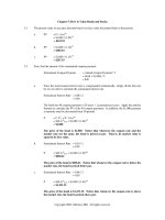
12.1 The discount rate for the project is equal to the expected return for the security, R
S
, since the
project has the same risk as the firm as a whole. Apply the CAPM to express the firm’s required
return, R
S
, in terms of the firm’s beta,
β
, the risk-free rate, R
F
, and the expected market return,

R
M
.

R
S
= R
F
+ β × (
R
M
– R
F
)
= 0.05 + 0.95 (0.09)
= 0.1355

Subtract the initial investment at year 0. To calculate the PV of the cash inflows, apply the
annuity formula, discounted at 0.1355.

NPV = C
0
+ C
1
A
T
r
= -$1,200,000 + $340,000 A
5
0.1355

= -$20,016.52

Do not undertake the project since the NPV is negative.

12.2 a. Calculate the average return for Douglas stock and the market.


R
D
= (Sum of Yearly Returns) / (Number of Years)
= (-0.05 + 0.05 + 0.08 + 0.15 + 0.10) / (5)
= 0.066


R
M

= (-0.12 + 0.01 + 0.06 + 0.10 + 0.05) / (5)
= 0.020

b. To calculate the beta of Douglas stock, calculate the variance of the market, (R
M
-
R
M
)
2
,
and the covariance of Douglas stock’s return with the market’s return, (R
D
-
R
D
) × (R
M
-
R
M
). The beta of Douglas stock is equal to the covariance of Douglas stock’s return and
the market’s return divided by the variance of the market.


R
D
-
R
D

R
M
-
R
M
(R
M
-
R
M
)
2
(R
D
-
R
D
) (R
M
-
R
M
)
-0.116 -0.14 0.0196 0.01624
-0.016 -0.01 0.0001 0.00016
0.014 0.04 0.0016 0.00056
0.084 0.08 0.0064 0.00672
0.034 0.03 0.0009 0.00102
0.0286 0.02470

β
D
= Cov (R
D
, R
M
) / Var (R
M
)
= (R
D
-
R
D
) (R
M
-
R
M
) / (R
M
-
R
M
)
2
= 0.02470 / 0.0286
= 0.864

The beta of Douglas stock is 0.864.

Copyright 2003, McGraw-Hill. All rights reserved.


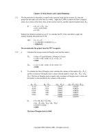
12.3 Calculate the square root of the stock’s variance and the market’s variance to find the standard
deviation, σ, of each.

σ
C
= (σ
2
C
)
1/2
= (0.004225)
1/2
= 0.065

σ
M
= (σ
2
M
)
1/2

= (0.001467)
1/2
= 0.0383

Use the formula for beta:

β
C
= [Corr (R
C
, R
M
) × σ
C
] / σ
M
= [(0.675) (0.065)] / (0.0383)
= 1.146

The beta of Ceramics Craftsman is 1.146.

12.4 a. To compute the beta of Mercantile’s stock, divide the covariance of the stock’s return
with the market’s return by the market variance. Since those two values are provided in
the problem, the 13 quarterly returns of Mercantile’s stock and the market are not needed
for the calculation.

β
D
= Cov (R
D

, R
M
) / σ
2
M
= (0.038711) / (0.038588)
= 1.0032

The beta of Mercantile Banking Corporation is 1.0032.

b. The beta of the average stock is one. Since Mercantile’s beta is close to one, its stock has
approximately the same risk as the overall market.

12.5 a. R
L
can have three values, 0.16, 0.18, or 0.20. The probability that R
L
takes one of these
values is the sum of the joint probabilities of the return pair, Prob(R
L
, R
J
), that includes
the particular value of R
L
. For example, if R
L
is equal to 0.16, R
J
will be either 0.16, 0.18,

or 0.22. The probability that R
L
is 0.16 and R
J
is 0.16 is 0.10. The probability that R
L
is
0.16 and R
J
is 0.18 is 0.06. The probability that R
L
is 0.16 and R
J
is 0.22 is 0.04. Thus,
the probability that R
L
assumes a value 0.16 is 0.20 (=0.10 + 0.06 + 0.04). The same
procedure is used to calculate the probability that R
L
is 0.18 and the probability that R
L
is
0.20.

R
L
Probability
0.16 0.20
0.18 0.60
0.20 0.20

b. i. The expected return on asset L is calculated by weighting each possible
return by its probability. Multiply each possible return, R
L
, by its probability, as
found in part (a).

R
L
= Σ[R
L
× Prob(R
L
)]
= (0.16)(0.20) + (0.18)(0.60) + (0.20) (0.20)
= 0.18

Copyright 2003, McGraw-Hill. All rights reserved.


The expected return on asset L is 18%.

ii. The variance of asset L is the weighted sum of the squared differences between
the possible values of R
L
and the expected return on R
L
found in part (i). Weight
the squared differences by the probabilities of each value found in part (a).

σ
2
L
= Σ[(R
L
-
R
L
)
2
× Prob(R
L
)]
= (0.16 – 0.18)
2
(0.20) + (0.18 – 0.18)
2
(0.60) + (0.20 – 0.18)
2
(0.20)
= 0.00016

The variance of asset L is 0.00016.

iii. The standard deviation of asset L is the square root of the variance calculated in
part (ii).

σ
L
= (σ

2
L
)
1/2
= (0.00016)
1/2

= 0.01265

The standard deviation of asset L is 0.01265.

c. Repeat the procedure used in part (a) to calculate the probability of each value of R
J
.

R
J
Probability
0.16 0.10
0.18 0.20
0.20 0.40
0.22 0.20
0.24 0.10

d. i. The expected return on asset J is the weighted probability of each possible
return. Multiply each possible return, R
J
, by the probability of each return found
in part (c).

R
J
= Σ[R
J
× Prob(R
J
)]
= (0.16)(0.10) + (0.18)(0.20) + (0.20)(0.40) + (0.22)(0.20) +
(0.24)(0.10)
= 0.20

The expected return on asset J is 20%.

ii. The variance of asset J is the weighted sum of the squared differences between
the possible values of R
J
and the expected return on R
J
found in part (i). Weight
the squared differences by the probabilities of each value found in part (c).

σ
2
J
= Σ[(R
J
-
R
J
)

2
× Prob(R
J
)]
= (0.16 – 0.20)
2
(0.10) + (0.18 – 0.20)
2
(0.20) + (0.20 – 0.20)
2
(0.40) +
(0.22 – 0.20)
2
(0.20) + (0.24 – 0.20)
2
(0.10)
= 0.00048

The variance of asset J is 0.00048.

iii. The standard deviation of asset J is the square root of the variance calculated in
part (ii).

Copyright 2003, McGraw-Hill. All rights reserved.


σ
J
= (σ
2

J
)
1/2
= (0.00048)
1/2
= 0.02191

The standard deviation of asset J is 0.02191.

d. The covariance is the expected value of [(R
L
-
R
L
) (R
J
-
R
J
)].

Cov (R
L
, R
J
) = Σ [(R
L
-
R
L

) × (R
J
-
R
J
) × Prob (R
L
, R
J
)]
= (0.16 – 0.18) (0.16 – 0.20) (0.10) + (0.16 – 0.18) (0.18 – 0.20) (0.06)
+ (0.16 – 0.18) (0.22 – 0.20) (0.04) + (0.18 – 0.18) (0.18 – 0.20) (0.12)
+ (0.18 – 0.18) (0.20 – 0.20) (0.36) + (0.18 – 0.18) (0.22 – 0.20) (0.12)
+ (0.20 – 0.18) (0.18 – 0.20) (0.02) + (0.20 – 0.18) (0.20 – 0.20) (0.04)
+ (0.20 – 0.18) (0.22 – 0.20) (0.04) + (0.20 – 0.18) (0.24 – 0.20) (0.10)
= 0.000176

The covariance of asset L’s return with asset J’s return is 0.000176.

The correlation coefficient of R
L
and R
J
is the covariance divided by the standard
deviation of assets L and J.

Corr (R
L
, R
J

) = Cov (R
L
, R
J
) / (σ
L
σ
J
)
= 0.000176 / (0.01265 × 0.02191)
= 0.635

The correlation coefficient of asset L and J is 0.635.

e. Divide the product of the correlation coefficient and the standard deviation of asset J by
the standard deviation of the market, asset L, to calculate the beta for asset J.

β
J
= [Corr (R
L
, R
J
) × σ
J
] / σ
L
= [(0.635) (0.02191)] / (0.01265)
= 1.10

The beta of asset J is 1.10.

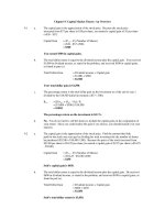
12.6 You are assuming that the new project’s risk is the same as the risk of the firm as a whole, and that
the firm is financed entirely with equity.

12.7 a. Jang Cosmetics should use its stock beta in the evaluation of the project only if the risk of
the perfume project is the same as the risk of Jang Cosmetics as a whole.

b. If the risk of the project is the same as the risk of the firm, use the firm’s stock beta.
Otherwise, Jang should use the beta of an all-equity firm that has similar risks as the
perfume project. An effective way to estimate the beta of the perfume project is to
average the betas of several all-equity, perfume-producing firms.

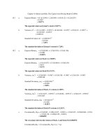
12.8 First, calculate the expected return on Compton’s stock.


R
S
= Σ[R
S
× Prob(R
S
)]
= (0.03) (0.1) + (0.08) (0.3) + (0.20) (0.4) + (0.15) (0.2)
= 0.137



Copyright 2003, McGraw-Hill. All rights reserved.

Calculate the expected return on Compton’s debt.


R
B
= Σ[R
B
B
× Prob(R
B
)]
= (0.08) (0.1) + (0.08) (0.3) + (0.1) (0.4) + (0.1) (0.2)
= 0.092

Calculate the expected return on the market.


R
M
= Σ[R
M
× Prob(R
M
)]
= (0.05) (0.1) + (0.1) (0.3) + (0.15) (0.4) + (0.2) (0.2)
= 0.135

Calculate the covariance of the stock’s return with the market’s return.

Cov (R
S
, R
M
) = Σ [(R
S
-
R
S
) × (R
M
-
R
M
) × Prob]
= (0.03 – 0.137) (0.05 – 0.135) (0.1) + (0.08 – 0.137) (0.1 – 0.135)
(0.3) + (0.2 – 0.137) (0.15 – 0.135) (0.4) + (0.15 – 0.137) (0.2 – 0.135)
(0.2)
= 0.002055

Calculate the covariance of the debt’s return with the market’s return.

Cov (R
B
, R
M
) = Σ [(R
B
-
R

B
) × (R
M
-
R
M
) × Prob]
= (0.08 – 0.092) (0.05 – 0.135) (0.1) + (0.08 – 0.092) (0.1 – 0.135)
(0.3) + (0.1 – 0.092) (0.15 – 0.135) (0.4) + (0.1 – 0.092) (0.2 – 0.135)
(0.2)
= 0.00038

Calculate the market variance.

σ
2
M
= Σ[(R
M
-
R
M
)
2
× Prob(R
M
)]
= (0.05 – 0.135)
2
(0.1) + (0.1 – 0.135)

2
(0.3) + (0.15 – 0.135)
2
(0.4) +
(0.2 – 0.135)
2
(0.2)
= 0.002025

a. Calculate the beta of Compton Technology’s debt by dividing the covariance of the
debt’s return with the market’s return by the variance of the market.

β
B
= Cov (R
B
, R
M
) / σ
2
M
= (0.00038) / (0.002025)
= 0.188

The beta of Compton Technology debt is 0.188.

b. Calculate the beta of Compton Technology’s stock by dividing the covariance of the
stock’s return with the market’s return by the variance of the market.

β

S
= Cov (R
S
, R
M
) / σ
2
M

= (0.002055) / (0.002025)
= 1.015

The beta of Compton Technology stock is 1.015.



Copyright 2003, McGraw-Hill. All rights reserved.