Tài liệu Enumeration of Kinematic Structures According to Function P4 ppt

Chapter 4
Structural Analysis of Mechanisms
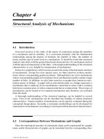
4.1 Introduction
Structural analysis is the study of the nature of connection among the members
of a mechanism and its mobility. It is concerned primarily with the fundamental
relationships among the degrees of freedom, the number of links, the number of
joints, and the type of joints used in a mechanism. It should be noted that structural
analysis only deals with the general functional characteristics of a mechanism and not
with the physical dimensions of the links. A thorough understanding of the structural
characteristics is very helpful for enumeration of mechanisms.
In this text, graph theory will be used as an aid in the study of the kinematic structure
of mechanisms. Except for a few special cases, we limit ourselves to those mecha-
nisms whose corresponding graphs are planar. Although there are a few mechanisms
whose corresponding graphs are not planar, these mechanisms usually contain a large
number of links. In addition, we also limit ourselves to graphs that contain no artic-
ulation points or bridges. A graph with an articulation point or a bridge represents a
mechanism that is made up of two mechanisms connected in series with a common
link but no common joint, or with a common joint but no common link. These types of
mechanisms can be treated as two separate mechanisms and, therefore, are excluded
from the study.
A thorough understanding of the structural topology can be helpful in several
ways. First of all, mechanisms can be classified into families of similar structural
characteristics. Various families of mechanisms can be quickly evaluated during the
conceptual design phase. Secondly, a systematic methodology can be developed for
enumeration of mechanisms according to certain prescribed structural characteristics.
4.2 Correspondence Between Mechanisms and Graphs
Since the topological structure of a kinematic chain can be represented by a graph,
many useful characteristics of graphs can be translated into the corresponding char-
© 2001 by CRC Press LLC
acteristics of a kinematic chain. Table 4.1 describes the correspondence between
the elements of a kinematic chain and that of a graph. Table 4.2 summarizes some

corresponding characteristics between kinematic chains and graphs.
Table 4.1
Correspondence Between Mechanisms and Graphs.
Graph Symbol Mechanism Symbol
Number of vertices
v
Number of links
n
Number of edges
e
Number of joints
j
Number of vertices of degree
iv
i
Number of links having
i
joints
n
i
Degree of vertex
id
i
Number of joints on link
id
i
Number of independent loops
L
Number of independent loops
L

Total number of loops (
L + 1
)
˜
L
Total number of loops (
L + 1
)
˜
L
Number of loops with
i
edges
L
i
Number of loops with
i
joints
L
i
Table 4.2
Structural Characteristics of Mechanisms and Graphs.
Graphs Mechanisms
L = e − v + 1 L = j − n + 1
e − v + 2 ≥ d
i
≥ 2 j − n + 2 ≥ d
i
≥ 2


i
d
i
= 2e

i
d
i
= 2j

i
v
i
= v

i
n
i
= n

i
iv
i
= 2e

i
in
i
= 2j
v

2
≥ 3v − 2en
2
≥ 3n − 2j

i
L
i
=
˜
L = L + 1

i
L
i
=
˜
L = L + 1

i
iL
i
= 2e

i
iL
i
= 2j
Isomorphic graphs Isomorphic mechanisms
4.3 Degrees of Freedom

The degrees of freedom of a mechanism is perhaps the first concern in the study of
kinematics and dynamics of mechanisms. The degrees of freedom of a mechanism
refers to the number of independent parameters required to completely specify the
configuration of the mechanism in space. Except for some special cases, it is possible
to derive a general expression for the degrees of freedom of a mechanism in terms
of the number of links, number of joints, and types of joints incorporated in the
mechanism. The following parameters are defined to facilitate the derivation of the
degrees of freedom equation.
© 2001 by CRC Press LLC
c
i
: degrees of constraint on relative motion imposed by joint i.
F : degrees of freedom of a mechanism.
f
i
: degrees of relative motion permitted by joint i.
j: number of joints in a mechanism, assuming that all joints are binary.
j
i
: number of joints with i dof; namely, j
1
denotes the number of 1-dof joints, j
2
denotes the number of 2-dof joints, and so on.
L: number of independent loops in a mechanism.
n: number of links in a mechanism, including the fixed link.
λ: degrees of freedom of the space in which a mechanism is intended to function.
It is assumed that a single value of λ applies to the motion of all the links of
a mechanism. For spatial mechanisms, λ = 6, and for planar and spherical
mechanisms, λ = 3. We call λ the motion parameter.

Intuitively, the degrees of freedom of a mechanism is equal to the degrees of
freedom of all the moving links diminished by the degrees of constraint imposed by
the joints. If all the links are free from constraint, the degrees of freedom of an n-link
mechanism with one link fixed to the ground would be equal to λ(n − 1). Since the
total number of constraints imposed by the joints are given by

i
c
i
, the net degrees
of freedom of a mechanism is
F = λ(n − 1) −
j

i=1
c
i
. (4.1)
The constraints imposed by a joint and the degrees of freedom permitted by the joint
are related by
c
i
= λ − f
i
. (4.2)
Substituting Equation (4.2) into Equation (4.1) yields
F = λ(n − j − 1) +
j

i=1

f
i
. (4.3)
Equation (4.3) is known as the Grübler or Kutzbach criterion [12]. In reality, the
criterion was established much earlier by Ball [4] and probably others. However,
unlike earlier researchers, Grübler and Kutzbach developed the equation specifically
for mechanisms.
The Grübler criterion is valid provided that the constraints imposed by the joints
are independent of one another and do not introduce redundant degrees of freedom.
A redundant degree of freedom is one that does not have any effect on the transfer
of motion from the input to the output link of a mechanism. For example, a binary
© 2001 by CRC Press LLC
link with two end spherical joints possesses a redundant degree of freedom as shown
in Figure 4.1. We call this type of freedom a passivedegreeoffreedom, because it
permits the binary link to rotate freely about a line passing through the centers of the
two joints with no torque transferring capability about that line.
FIGURE 4.1
AnS–Sbinary link.
In general, a binary link with either S−S, S−E,orE−E pairs as its end
joints possesses one passive degree of freedom as outlined in Table 4.3. In addition,
a sequence of binary links with S − S, S − E,orE − E pairs as their terminal joints
also possess a passive degree of freedom.
Table 4.3
Binary Links with Passive Degrees of Freedom.
End Joints Passive Degree of Freedom
S − S
Rotation about an axis passing through the centers of the two ball joints.
S − E
Rotation about an axis passing through the center of the ball and per-
pendicular to plane of the plane pair.

E − E
Sliding along an axis parallel to the line of intersection of the planes of
the two E pairs. If the two planes are parallel, three passive dof exist.
Passive degrees of freedom cannot be used to transmit motion or torque about
an axis. When such joint pairs exist, one degree of freedom should be subtracted
from the degrees of freedom equation. We exclude the E − E combination as being
impractical, because a link (or links) with an E − E pair can slide freely along an
axis parallel to the line of intersection of the two E planes. Let f
p
be the number of
passive degrees of freedom in a mechanism, then Equation (4.3) can be modified as
F = λ(n − j − 1) +
j

i=1
f
i
− f
p
. (4.4)
© 2001 by CRC Press LLC
In general, if the Grübler criterion yields F>0, the mechanism has F degrees
of freedom. If the criterion yields F = 0, the mechanism becomes a structure with
zero degrees of freedom. On the other hand, if the criterion yields F<0, the mech-
anism becomes an overconstrained structure. It should be noted, however, that there
are mechanisms that do not obey the degrees of freedom equation. These overcon-
strained mechanisms require special link length proportions to achieve mobility. The
Bennett [5] mechanism is a well-known overconstrained spatial 4R linkage. It con-
tains four links connected in a loop by four revolute joints. The opposite links have
equal link lengths and twist angles, and are related to that of the adjacent link by a

special condition. According to Equation (4.3), the degrees of freedom of the Ben-
net mechanism should be equal to −2. In reality, the mechanism does possess one
degree of freedom. Other well-known overconstrained mechanisms include the Gold-
berg [10] five-bar and Bricard six-bar linkages. Recently, Mavroidis and Roth [13]
developed an excellent methodology for the analysis and synthesis of overconstrained
mechanisms. Many previously known and new overconstrained mechanisms can be
found in that work. This text is not concerned with overconstrained mechanisms.
Example 4.1 Planar Three-Link Chain
For the planar three-link, 3R kinematic chain shown in Figure 4.2, we haven= 3
and j = j
1
= 3. Equation (4.3) yields F = 3(3 − 3 − 1) + 3 = 0. Hence, a planar
three-link chain connected by revolute joints is a structure. Three-link structures can
be found in many civil engineering applications.
FIGURE 4.2
Three-bar structure.
Example 4.2 Planar Four-Bar Linkage
For the planar four-bar, 4R linkage shown in Figure 1.8, we have n= 4 and
j = j
1
= 4. Equation (4.3) yields F = 3(4 − 4 − 1) + 4 = 1. Hence, the planar
four-bar linkage is a one-dof mechanism.
© 2001 by CRC Press LLC
Example 4.3 Planar Five-Bar Linkage
For the planar five-bar, 5R linkage shown in Figure 4.3, we have n= 5 and
j = j
1
= 5. Equation (4.3) gives F = 3(5 − 5 − 1) + 5 = 2. Hence, the planar
five-bar linkage is a two-dof mechanism.
FIGURE 4.3

Five-bar linkage.
Example 4.4 Spur-Gear Drive
For the spur-gear set shown in Figure 1.10, we have n= 3 and j
1
= 2,j
2
= 1.
Equation (4.3) gives F = 3(3 − 3 − 1) + 4 = 1. Therefore, the spur-gear drive is a
one-dof mechanism.
Example 4.5 Spatial RCSP Mechanism
For the spatial RCSP mechanism shown in Figure 3.17, we have n= 4,j
1
=
2,j
2
= 1, and j
3
= 1. Equation (4.3) yields F = 6(4−4−1)+2×1+1×2+1×3 = 1.
Hence, the RCSP linkage is a one-dof mechanism.
Example 4.6 Swash-Plate Mechanism
For the swash-plate mechanism shown in Figure 1.12, we have n= 4,j
1
=
2,j
2
= 0,j
3
= 2,j= j
1
+ j

3
= 4, and f
p
= 1. Equation (4.4) gives
F = 6(4 − 4 − 1) + 2 × 1 + 2 × 3 − 1 = 1.
Both the RCSP and swash-plate mechanisms can be designed as a compressor or
engine mechanism.
© 2001 by CRC Press LLC
4.4 Loop Mobility Criterion
In the previous section, we derive an equation that relates the degrees of freedom
of a mechanism to the number of links, number of joints, and type of joints. It is also
possible to establish an equation that relates the number of independent loops to the
number of links and number of joints in a kinematic chain.
The four-bar linkage shown in Figure 1.8 is a single-loop kinematic chain having
four links connected by four joints. The five-bar linkage shown in Figure 4.3 is also
a single-loop kinematic chain. It is made up of five links connected by five joints.
We observe that for a single-loop kinematic chain (planar, spherical, or spatial), the
number of joints is equal to the number of links (n = j ), and the links are all binary.
We now extend a single-loop chain to a two-loop chain. This can be accomplished
by taking an open-loop chain and joining its two ends to members of a single-loop
chain by two joints as shown in Figure 4.4. We observe that by extending from a
FIGURE 4.4
Formation of a multiloop chain.
one- to two-loop chain, the number of joints added is more than the number of links
by one. Similarly, an open-loop chain can be added to a two-loop chain to form a
three-loop chain, and so on. By induction, extending a kinematic chain from 1 to L
loops, the difference between the number of joints and number of links is increased
by L − 1. Therefore,
L = j − n + 1 . (4.5)
Or, in terms of the total number of loops, we have

˜
L = j − n + 2 . (4.6)
© 2001 by CRC Press LLC
Equation (4.5) is known as Euler’s equation. Combining Equation (4.5) with Equa-
tion (4.3) yields
j

i=1
f
i
= F + λL . (4.7)
Equation (4.7) is known as the loop mobility criterion. The loop mobility criterion is
useful for determining the number of joint degrees of freedom needed for a kinematic
chain to possess a given number of degrees of freedom.
Example 4.7 Four-Bar Linkage
For the planar four-bar linkage shown in Figure 1.8, we have n= 4,j= 4.
Equation (4.5) yields L = 1. For F = 1, Equation (4.7) yields

f
i
= 1+3×1 = 4.
Hence, the total number of joint degrees of freedom should be equal to four to achieve
a one-dof mechanism.
Example 4.8 Humpage Gear Reducer
The Humpage gear reduction unit shown in Figure 3.14 is a five-bar spherical
mechanism, in which links 1, 2, and 5 are three coaxial bevel gears, link 3 is a
compound planet gear, and link 4 is the carrier. In this mechanism, link 1 is fixed
to the ground, link 5 is the input link, and link 2 serves as the output link. The
compound planet gear 3 meshes with gears 1, 2, and 5. Overall, the mechanism has
four revolute joints and three gear pairs. With λ = 3, n = 5,j

1
= 4,j
2
= 3, and
F = 1, Equation (4.5) yields L = 3 and Equation (4.7) yields

f
i
= 10.
4.5 Lower and Upper Bounds on the Number of Joints on a Link
Since we are interested primarily in nonfractionated closed-loop chains, every link
should be connected to at least two other links. Let d
i
denote the number of joints on
link i. The lower bound on d
i
is
d
i
≥ 2 . (4.8)
The upper bound on d
i
can be established from graph theory. Using the fact that the
number of loops of which a vertex is a part is equal to its degree, and the maximum
degree of a vertex is equal to the total number of loops, we have
˜
L ≥ d
i
, (4.9)
© 2001 by CRC Press LLC

where
˜
L = L + 1. Combining Equations (4.8) and (4.9) yields
˜
L ≥ d
i
≥ 2 . (4.10)
In other words, the minimum number of joints on each link of a closed-loop chain
is 2 and the maximum number is limited by the total number of loops.
Example 4.9 Stephenson Six-Bar Linkage
Figure4.5showsthekinematicstructureandgraphrepresentationoftheStephenson
six-bar linkage. The number of joints on the links are: d
1
= d
3
= d
4
= d
6
= 2, and
d
2
= d
5
= 3. Since there are six links and seven joints, the number of independent
loops is given by L = j − n + 1 = 7 − 6 + 1 = 2. Hence, the number of joints on
any link is bounded by 3 ≥ d
i
≥ 2.
FIGURE 4.5

Stephenson six-bar linkage.
Since each joint connects two links, we have
n

i=1
d
i
= d
1
+ d
2
+···+d
n
= 2j. (4.11)
Equation (4.11) is equivalent to Equation (2.4) derived in Chapter 2. Given the number
of joints, Equation (2.4) can be solved for various vertex-degree listings. The solution
can be regarded as the number of combinations with repeats permitted of n things
taken 2j at a time, subject to the constraint imposed by Equation (4.10) [11]. Since

i
d
i
over vertices of even degree and 2j are both even numbers, we conclude that
the number of links in a mechanism with an odd number of joints is an even number.
© 2001 by CRC Press LLC
4.6 Link Assortments
Links in a mechanism can be grouped according to the number of joints on them.
A link is called a binary, ternary, or quaternary link depending on whether it has two,
three, or four joints. Figure 4.6 shows the graph and kinematic structural representa-
tions of the above three links.

FIGURE 4.6
Binary, ternary, and quaternary links.
Let n
i
denote the number of links with i joints, that is, n
2
denotes the number of
binary links, n
3
the number of ternary links, n
4
the number of quaternary links, and
so on. Clearly,
n
2
+ n
3
+ n
4
+···+n
r
= n, (4.12)
where r =
˜
L denotes the largest number of joints on a link.
Since each of the n
i
links contains i joints and each joint connects exactly two
links, the following equation holds.
2n

2
+ 3n
3
+ 4n
4
+···+rn
r
= 2j. (4.13)
Equations (4.12) and (4.13) are equivalent to Equations (2.8) and (2.9) derived in
Chapter 2.
Multiplying Equation (4.12) by 3 and subtracting Equation (4.13), we obtain
n
2
= 3n − 2j +
(
n
4
+ 2n
5
+···
)
. (4.14)
© 2001 by CRC Press LLC
Therefore, the lower bound on the number of binary links is
n
2
≥ 3n − 2j. (4.15)
Given the number of links and the number of joints, Equations (4.12) and (4.13)
can be solved for all possible combinations of n
2

,n
3
,...,n
r
. All solutions, however,
must be nonnegative integers. The number of solutions can be treated as the number
of partitions of the integer 2j into parts 2, 3, ...,r with repetition permitted. This is a
well-known problem in combinatorial analysis. The solutions can be found by using
a nested-do loops computer algorithm to vary the values of n
i
. See Appendix A for a
description of the method. In the following, we study a heuristic algorithm developed
by Crossley [8].
1. Given the number of links and the number of joints, find the upper and lower
bounds on the number of joints on a link by Equation (4.10), and the minimal
number of binary links by Equation (4.15).
2. Find a particular solution to Equations (4.12) and (4.13). This can be done by
equating all but two variables, say n
2
and n
3
, to zero and solving the resulting
equations for these two variables. This produces one solution called a link
assortment.
3. For the link assortment obtained in the preceding step, apply Crossley’s op-
erator, (1, −2, 1) or its negative, wherever possible, to any three consecutive
numbers of n
i
s. Crossley’s operator effectively adds one link with i − 1 joints,
subtracts two links with i joints, and then adds another link with i + 1 joints.

The operation does not affect the identities of Equations (4.12) and (4.13). Fur-
thermore, a double application of the operator to any four consecutive n
i
s with
an offset is equivalent to the application of a (1, −1, −1, 1) operator which,
therefore, can be used alternatively.
4. Repeat Step 3 as many times as needed until all the possible assortments are
found.
For the purpose of classification, each link assortment is called a family. Each
family is identified by a vertex degree listing. The vertex degree listing is defined as
a list of integers representing the number of vertices of the same degree in ascending
order. Specifically, in the vertex degree listing, the first digit represents the number of
binary links, the second the number of ternary links, the third the number of quaternary
links, and so on. For example, a kinematic chain with n
2
= 4,n
3
= 1,n
4
= 3, and
n
5
= 2 (or in terms of a graph there are 4 vertices of degree two, 1 vertex of degree
three, 3 vertices of degree four, and 2 vertices of degree five) has a vertex degree
listing of “4132.”
Example 4.10 Link Assortments of (8, 10) Kinematic Chains
We wish to find all possible link assortments for planar kinematic chains with n = 8
and j = 10. Applying Equation (4.6), the upper bound on the number of joints on a
© 2001 by CRC Press LLC
link is 4. From Equation (4.15), the lower bound on the number of binary links is 4.

Hence, with n = 8 and j = 10, Equations (4.12) and (4.13) reduce to
n
2
+ n
3
+ n
4
= 8 , (4.16)
2n
2
+ 3n
3
+ 4n
4
= 20 . (4.17)
A particular solution to Equations (4.16) and (4.17) is found to be n
2
= 4,n
3
= 4,
and n
4
= 0. Applying Crossley’s operator, we obtain the following three families of
link assortments:
Family
n
2
n
3
n

4
4400 4 4 0
5210 5 2 1
6020 6 0 2
The 4400 family is made up of 4 binary and 4 ternary links; the 5210 family consists
of 5 binary, 2 ternary, and 1 quaternary links; and the 6020 family is composed of
6 binary and 2 quaternary links.
The above solutions can also be treated as a problem of solving a system of 2
linear equations in 3 unknowns, subject to the constraints that n
2
,n
3
, and n
4
must
be nonnegative integers and that n
2
≥ 4. Subtracting 2 × Equation (4.16) from
Equation (4.17), we obtain
n
3
+ 2n
4
= 4 . (4.18)
Equation (4.18) contains two unknowns. Since both 2n
4
and 4 are even numbers, n
3
must be an even number. Let n
3

assume the values of 0, 2, and 4, one at a time, then
n
4
= 2, 1, and 0, respectively. Once n
3
and n
4
are known, we solve Equation (4.16)
for n
2
. This leads to the same results.
4.7 Partition of Binary Link Chains
Binary links in a mechanism may be connected in series to form a binary link chain.
The first and last links of a binary link chain are necessarily connected to nonbinary
links. We define the length of a binary link chain by the number of binary links in
that chain. Furthermore, we consider the special case for which two nonbinary links
are connected directly to each other as a binary link chain of zero length. Binary link
chains of length 0, 1, 2, and 3 are called the E, Z, D, and V chains, respectively, as
depicted in Figure 4.7.
Let b
k
denote the number of binary link chains of length k, and q denote the
maximal length of a binary link chain in a kinematic chain. Applying Equations (2.39)
© 2001 by CRC Press LLC
FIGURE 4.7
Various binary link chains.
and (2.40), we obtain
b
1
+ 2b

2
+ 3b
3
+···+qb
q
= n
2
, (4.19)
b
0
+ b
1
+ b
2
+ b
3
+···+b
q
= j − n
2
. (4.20)
The length of a binary link chain is limited by the fact that the degrees of freedom
associated with a binary link chain must be less than that of the mechanism as a whole.
A binary link chain of length k contains k binary links and k + 1 joints. If the links
and joints of a binary link chain were independently movable with F -dof relative to
the rest of the mechanism, Equation (4.7) would lead to
k+1

i=1
f

i
= F + λ,
where

k+1
i=1
f
i
denotes the total joint degrees of freedom associated with a binary
link chain of length k. It follows that the remaining links and joints of the mechanism
© 2001 by CRC Press LLC
would be overconstrained. Therefore, to avoid such degenerate cases, we impose the
condition
k+1

i=1
f
i
≤ F + λ − 1 . (4.21)
The maximum number of joints occurs when all the joints in a binary link chain are
one-dof joints. It follows from Equation (4.21) that the length of a binary link chain
is limited by
q ≤ F + λ − 2 . (4.22)
For each family of link assortment, we can solve Equations (4.19) and (4.20)
for various combinations of binary link chains. Since Equation (4.20) contains one
more variable than that of Equation (4.19), we can solve Equation (4.19) for b
k
for
k = 1, 2,...,q, and then Equation (4.20) for b
0

. The solution to Equation (4.19) can
be regarded as the number of partitions of the integer n
2
into parts 1, 2,...,q with
repetition allowed. We can employ a nested-do loops computer algorithm to vary the
value of each b
k
to search for all feasible solutions. We call each solution set of b
k
a
branch. Thus a family of binary link assortment may produce several branches.
Example 4.11 Partition of Binary Links for the (8, 10) Kinematic Chains
We wish to identify all possible partitions of the binary links associated with the
(8, 10) planar kinematic chains derived in the preceding section. Assuming F = 1,
Equation (4.22) gives
q ≤ 2
as the upper bound on the length of a binary link chain.
4400 family: The 4400 family contains 4 binary links. Hence, Equations (4.19)
and (4.20) reduce to
b
1
+ 2b
2
= 4 , (4.23)
b
0
+ b
1
+ b
2

= 6 . (4.24)
Solving Equation (4.23) for nonnegative integers of b
1
and b
2
, and then Equa-
tion (4.24) for b
0
yields
Branch
b
0
b
1
b
2
1402
2321
3240
Hence, there are three branches of binary link chains. The first branch consists of
no binary link chains of length 1 and two binary link chains of length 2; the second
© 2001 by CRC Press LLC