THE LINEAR REGRESSION ANH RELATED STATISTICAL MODELS
Bạn đang xem bản rút gọn của tài liệu. Xem và tải ngay bản đầy đủ của tài liệu tại đây (693.37 KB, 19 trang )
PART
IV
The linear regression and related statistical
models
CHAPTER
17
Statistical models
17.1
in econometrics
Simple statistical models
The main purpose of Parts I] and III has been to formulate and discuss the
concept of a statistical model which will form the backbone of the
discussion in Part IV. A statistical model has been defined as made up of
two related components:
(i)
a probability model, ®= {D(y; 0), @¢ O}+ specifying a parametric
family of densities indexed by 0; and
a sampling model, y=(y;, ¥2,---. Jr)’ defining a sample from
D(y; 69), for some ‘true’ @ in O.
The probability model provides the framework in the context of which the
stochastic environment of the real phenomenon being studied can be
(ii)
defined and the sampling model describes the relationship between the
probability model and the observable data. By postulating a statistical
model we transform the uncertainty relating to the mechanism giving rise to
the observed data to uncertainty relating to some unknown parameter(s) 0
whose estimation determines the stochastic mechanism D(y; 6).
An example of such a statistical model in econometrics is provided by the
modelling of the distribution of personal income. In studying the
distribution of personal income higher than a lower limit yy the following
statistical model is often postulated:
0
Yo
“)
yh
8+1
(i)
D= 4 D(y/yos A=
(1)
y=(¡.ÿ¿,..., Yy) isa random
+0
J
0cf`,,
y>yo¿:
sample from D(y/ya;0).
+ The notation in Part IV will be somewhat different from the one used in Parts Il and
IH. This change in notation has been made
econometric notation.
339
to conform with the established
340
Statistical models in econometrics
Note:
Eu=r(
0\
jo 3)
.
if 8> Ì,
Vary)=yjÍ——„5—-Ì.J it o>2
YOK = 10-2)
For y a random sample the likelihood function is
/Ø0N(y,V*!
T
=0 y,,y;,..., vợ) 690,
LỊU; y)= H (2?)
t=1 XŸo/
Vi
r
log L(6; y)= T log 0+ TO log yy —(0+ 1) ¥ log y,,
dlogL
ẽ
dé)
is the maximum
t=1
T
— + T log yo — >. log y,=0,
t
0=r| ("||
likelihood
estimator (MLE)
of the parameter
6. Since
(d? log L)/d6? = — T/6?, the asymptotic distribution of6 takes the form (see
Chapter
13):
/ T(8— 0) ~ NI0, 0°).
Although in general the finite sample distribution is not frequently
available, in this particular case we can derive D(0) analytically. It takes the
form
Ö
T-ITT-I
D())=—
(Ø) rt
T0
: | ~—},
-)
) >0.
ie.| (
ie
2T9
—-]~z?2T
5 ) x27)
(see Appendix 6.1). This distribution of § can be used to consider the finite
sample properties of 0 as well as test hypotheses or set up confidence
intervals for the unknown parameter 0. For instance, in view of the fact that
E(6) = (¿;}"
we can deduce that Ô is a biased estimator of 0.
It is of interest in this particular case to assess the ‘accuracy’ of the
asymptotic distribution of @ for a small T, (T=8), by noting that
^
T?8?
¬-.=
17.1
Simple statistical models
341
(see Johnson and Kotz (1970)). Using the data on income distribution (see
Chapter 2), for y> 5000 (reproduced below) to estimate 0,
Income lower
limit
No. of
incomes
5000
6000
7000
8000
10 000
12 000
15000
20 000
2600
1890
1150
990
410
220
100
50
we get
aap
as the ML
loe(**) | = 1.6
estimate.
Using the invariance property of MLE’s (see Section 13.3) we can deduce
that
£(0)=2.13,
Var(6)=0.91.
As we can see, for a small sample (T=8) the estimate of the mean and the
variance are considerably larger than the ones given by the asymptotic
distribution:
a
2
0Ậ2
E(O}= 1.6, Var(t) =; = 0.32.
On the other hand, for a much larger sample, say T= 100,
E(6)= 1.63,
Var(6)=0.028,
as compared with
E(6)=1.6,
Var(0)=0.026.
These results exemplify the danger of
samples and should be viewed as a
asymptotic theory. For a more general
how to improve upon the asymptotic
using asymptotic results for small
warning against uncritical use of
discussion of asymptotic theory and
results see Chapter 10.
The statistical inference results derived above in relation to the income
distribution example depend crucially on the appropriateness of the
statistical model postulated. That is, the statistical model should represent a
good approximation of the real phenomenon to be explained in a way
which takes account the nature of the available data. For example, if the
data were collected using stratified sampling then the random sample
assumption is inappropriate (see Section 17.2 below). When any of the
342
Statistical models in econometrics
assumptions
underlying
the
statistical
model
are
invalid
the
above
estimation results are unwarranted.
In the next three sections it is argued that for the purposes of econometric
modelling we need to extend the simple statistical model based on a random
sample, illustrated above, in certain specific directions as required by the
particular features of econometric modelling. In Section 17.2 we consider
the nature of economic data commonly available and discuss its
implications for the form of the sampling model. It is argued that for most
forms of economic data the random sample assumption is inappropriate.
Section 17.3 considers the question of constructing probability models if the
identically distributed assumption does not hold. The concept of a
statistical generating mechanism (GM) is introduced in Section 17.4 in
order to supplement the probability and sampling models. This additional
component enables us to accommodate certain specific features of
econometric modelling. In Section 17.5 the main statistical models of
interest in econometrics are summarised
which follows.
17.2
as a prelude to the discussion
Economic data and the sampling model
Economic data are usually non-experimental in nature and come in one of
three forms:
(i)
time Series, Measuring a particular variable at successive points in
time (annual, quarterly, monthly or weekly);
(ii)
cross-section, measuring a particular variable at a given point in
time over different units (persons, households, firms, industries,
countries, etc.);
(1)
panel data, which refer to cross-section data over time.
Economic data such as M1 money stock (M), real consumers’ expenditure
(Y) and its implicit deflator (P), interest rate on 7 days’ deposit account (J),
over time, are examples of time-series data (see Appendix, Table 17.2). The
income data used in Chapter 2 are cross-section data on 23 000 households
in the UK for 1979-80. Using the same 23 000 households of the crosssection observed over time we could generate panel data on income. In
practice, panel
data
are rather
rare in econometrics
because
of the
difficulties involved in gathering such data. For a thorough discussion of
econometric modelling using panel data see Chamberlain (1984).
The econometric modeller is rarely involved directly with the data
collection and refinement and often has to use published data knowing very
little about their origins. This lack of knowledge can have serious
repercussions on the modelling process and lead to misleading conclusions.
Ignorance related to how the data were collected can lead to an erroneous
17.2,
Economic data and the sampling model
343
choice of an appropriate sampling model. Moreover, if the choice of the
data is based only on the name they carry and not on intimate knowledge
about what exactly they are measuring, it can lead to an inappropriate
choice of the statistical GM
(see Section
17.4, below) and some misleading
conclusions about the relationship between the estimated econometric
model and the theoretical model as suggested by economic theory (see
Chapter 1). Let us consider the relationship between the nature of the data
and the sampling model in some more detail.
In Chapter 11 we discussed three basic forms of a sampling model:
(i)
random sample — a set of independent and identically distributed
(ID) random variables (r.v.’s);
(ii)
independent sample — a set of independent but not identically
distributed r.v.’s; and
(iit)
non-random sample — a set of non-IID r.v.’s.
For cross-section data selected by the simple random sampling method
(where every unit in the target population has the same probability of being
selected), the sampling model of a random sample seems the most
appropriate choice. On the other hand, for cross-section data selected by
the stratified sampling method (the target population divided into a
number of groups (strada) with every unit in each group having the same
probability of being selected), the identically distributed assumption seems
rather inappropriate. The fact that the groups are chosen a priori in some
systematic
way
renders
the
identically
distributed
assumption
inappropriate. For such cross-section data the sampling model of an
independent
sample
seems
more
appropriate.
The
independence
assumption can be justified if sampling within and between groups is
random.
For time-series data the sampling models ofa random or an independent
sample seem rather unrealistic on a priori grounds, leaving the non-random
sample as the most likely sampling model to postulate at the outset. For the
time-series data plotted against time in Fig. 17. 1(a)-(d) the assumption that
they represent realisations of stochastic processes (see Chapter 8) seems
more realistic than their being realisations of IID r.v.’s. The plotted series
exhibit considerable time dependence. This is confirmed in Chapter 23
where these series are used to estimate a money adjustment equation. In
Chapters
19-22
the
sampling
model
of
an
independent
sample
is
intentionally maintained for the example which involves these data series
and several misleading conclusions are noted throughout.
In order to be able to take explicitly into consideration the nature of the
observed data chosen in the context of econometric modelling, the statistical
models of particular interest in econometrics will be specified in terms of the
observable r.v.’s giving rise to the data rather than the error term, the usual
344
Statistical models in econometrics
35000 |-
§=
E
a
=
25000 |-
15000 |-
5000 Wubitiitliiithii
iti ditt td
1963
1966
1969
1972
1975
1978
1982
1975
1978
1982
Time
(a)
18000 |-
=
2 16000 Ƒ-
E
a
`
14000 |-
12000
1963
1966
1969
1972
Time
(b)
Fig. 17.1(a).
Money stock £(million). (b) Real consumers’ expenditure.
approach in econometrics textbooks (see Theil (1971), Maddala (1977),
Judge et al. (1982) inter alia). The approach adopted in the present book is
to extend the statistical models considered so far in Part HI in order to
accommodate certain specific features of econometric modelling. In
particular a third component, called a statistical generating mechanism
(GM) will be added to the probability and sampling models in order to
enable us to summarise the information involved in a way which provides
17.2.
Economic data and the sampling model
345
240 —
200 |-
160
Pd
ar
120 |-
80_—
49
1963
Todds
1966
tated
1969
teva t et
1972
de
1975
1978
1982
Time
(c)
tiiliiiliirliiiliirliirliiiiliiirLiiiliirliiicLiiiLiiriliiiriiiiLiyiliiiEiiilittLiti
1963
(d)
1966
1969
1972
1975
1978
1982
Time
Fig. 17.1(c).
Implicit price deflator. (d) Interest rate on 7 days’ deposit
account.
‘an adequate’ approximation to the actual DGP giving rise to the observed
data (see Chapter 1). This additional component will be considered
extensively in Section 17.4 below. In the next section the nature of the
probabiiity models required in econometric modelling will be discussed in
view of the above discussion of the sampling model.
346
Statistical models in econometrics
17.3
Economic data and the probability model
In Chapter | it was argued that the specification of statistical models should
take account not only of the theoretical a priori information available but
the nature of the observed data chosen as well. This is because the
specification of statistical models proposed in the present book is based on
the observable random variable giving rise to the observed data and not by
attaching a white-noise error term to the theoretical model. This strategy
implies
that
the
modeller
should
consider
assumptions
such
as
independence, stationarity, mixing (see Chapter 8) in relation to the
observed data at the outset.
As argued in Section 17.2, the sampling model ofa random sample seems
rather unrealistic for most situations in econometric modelling in view of
the economic
data usually available.
Because of the interrelationship
between the sampling and the probability model we need to extend the
simple probability model ®={D(y; 6), 0¢@} associated with a random
sample to ones related to independent and non-random samples.
An independent (but non-identically distributed) sample y=(y,,.... Vr)
raises questions of time-heterogeneity in the context of the corresponding
probability model. This is because in general every element }, of y has its
own distribution with different parameters D(y,; 0,). The parameters 6,
which depend on t are called incidental parameters. A probability model
related to y takes the general form
(17.1)
D= {D(y,; 8,), 6, €®, te T},
where T={1, 2,...} is an index set.
A non-random sample y raises questions not only of time-heterogeneity
but of time-dependence as well. In this case we need the joint distribution ofy
in order to define an appropriate probability model of the general form
®=D(y¿,y;,...,
vr: 6y), 0;e@, T,=(1,2,...,7)ST}.
(172)
In both of the above cases the observed data can be viewed as realisations
of the stochastic process {y,,t¢ T} and for modelling purposes we need to
restrict its generality using assumptions such as normality, stationarity and
asymptotic independence or/and supplement the sample and theoretical
information available. In order to illustrate these let us consider the
simplest case of an independent sample and one incidental parameter:
0
:
9=iturznaslaf2"jk
ly
—u
6,=(u,,ø?)elRx R„, ret
17.3.
(ii)
The
Data and the probability model
347
Y=(V¡,Y¿...., yr} 1s an independent sample from D(y,; 6,),¢= 1, 2,
..., T, respectively.
probability
model
postulates
a normal
density
with
mean
yp, (an
incidental parameter) and variance o?. The sampling model allows each y, to
have a different mean but the same variance and to be independent of the
other y,s. The distribution of the sample for the above statistical model
D(y: 6) where y=(y1, y„..... yr) and Ð=(H, Hạ,..., Hạ, Ø7) 1s
Diy, 0)= [] Dữ tụ, ở)
t=1
1
T
=(ø?)T2(2m)*” exp) —>
À, w-wh
20°
(17.3)
424
As we can see, there are T+ 1 unknown parameters, 0= (07, Hy, 2... 5 Hr)s
to be estimated and only T observations which provide us with sufficient
warning that there will be problems. This is indeed confirmed by the
maximum likelihood (ML) method. The log likelihood is
T
1
2
2
20°
24
log L(6; y)=const—— logø?—— 3` (y—MjŸ,
elog
ob
L
1
(—2)(y,—m)=0,
Ch,
t=1,2,...,T,
2ø
Clog L
T
1
Oe “=——~13——~
2g212g4
6a2
ÈÚ,
—
3
Hạ)
(174)
(175)
=0.0
(
17.6
)
These first-order conditions imply that f,=y,,t=1,2,..., T, and 6?=0.
Before we rush into pronouncing these as MLE'’s it is important to look at
the second-order conditions for a maximum.
=_+
é7 log L
é? log L
oc?
ơm;
fy
ỡae
ag?
Gat
T
1
2308820
Ly)
2
ở
tị” Hy
ø?=¿?
which are unbounded and hence đ, and ô? are not MLE”s; see Section 13.3.
This suggests that there is not enough information in the statistical model
(i)(ii) above to estimate the statistical parameters 0=(y,, HU, .-., ps 0”).
An obvious way to supplement this information is in the form of panel
data for y,, say y,,i=1,2,...,N,t=1,2,..., T. In the case where N
realisations of y, are available at each t, 8 could be estimated by
.
1
N
32 Đề
ly N 24
t=1,2,...,T
(172)
348
Statistical models in econometrics
and
(178)
1z
1i
II
I*⁄¬
=+1 > 3> 0w=8)Ẻ
P=
1
It can be verified that these are indeed the MLE’s of Ø.
An alternative way to supplement the information of the statistical model
{i){il) is to reduce the dimensionality of the statistical parameter space ©.
This can be achieved by imposing restrictions on 8 or modelling @ by
relating it to other observable random variables (r.v.’s) via conditioning (see
Chapter 7). Note that non-stochastic variables are viewed as degenerate
r.v.’s. The latter procedure enables us to accommodate theoretical
information within a probability model by relating such information to the
Statistical parameters @. In particular, such information is related to the
mean (marginal or conditional) of r.v.’s involved and sometimes to the
variance.
Theoretical
information
is
rarely
related
to
higher-order
moments (see Chapter 4).
The modelling of statistical parameters via conditioning leads naturally
to an additional component to supplement the probability and sampling
models. This additional component we call a statistical generating
mechanism (GM) for reasons which will become apparent in the discussion
which follows. At this stage it suffices to say that the statistical GM
is
postulated as a crude approximation to the actual DGP which gave rise to
the observed data in question, taking account of the nature af such data as
well as theoretical a priori information.
In
the case of the
statistical
model
(i)}-(ii) above
we
could
‘solve’ the
inadequate information problem by relating , to a vector of observable
variables x4,, X2,-.-, Xig, f=1,2,..., T, say, linearly, to postulate
Li, =b'x,,
(17.9)
where b=(b,, b>, ..., b,)', K
postulating this relationship we reduce the parameter space from
O=R’x R, and increasing with T to @,=R* x R., and independent of T.
The statistical GM in this case takes the general form
y,=b’x,+u,,
teT,
(17.10)
where y,=b’x, and u,= y,—b’x, are called systematic and non-systematic
components of y,, respectively. By construction
E(uu,)=0
and
Elu,)=0,
EluZ)=o*,
E(u,u,)=0,
tés,
tse,
where E(-) is defined relative to D(y,; 0), the marginal distribution of y,.
Equation (10) represents a situation where the choice of the values x;,, Xạ,,
17.4
The statistical generating mechanism
...„X„; determines the systematic part of y, with
being a white-noise process (see Chapter 8). This is
Gauss linear model (see Chapter 18). The above
extended in the next section in order to define some
statistical models in econometrics.
17.4
349
the unmodelled part u,
the statistical GM of the
statistical GM will be
of the most widely used
The statistical generating mechanism
The concept ofa statistical GM is postulated to supplement the probability
and sampling models and represents a crude approximation to the actual
DGP which gave rise to the available data. It represents a summarisation of
the sample information in a way which enables us to accommodate any a
priori information related to the actual DGP as suggested by economic
theory (see Chapter 1).
Let {y,,t€ 1} be a stochastic process defined on (S, F P(-)) (see Chapter
8). The statistical GM
}¿=H,+u,
is defined by
cet,
(17.11)
where
u=E\y,2),
GoF,
(17.12)
2 being some ø-field. Thịs defines the statistical process generating y, with
Ht, being the postulated systematic mechanism giving rise to the observed
data on y, and u, the non-systematic part of y, defined by u,=y,—4,.
Defining u, this way ensures that it is orthogonal to the systematic
component p,; denoted by y,Lu, (see Chapter 7). The orthogonality
condition is needed for the logical consistency of the statistical GM in view
of the fact that u, represents the part of y, left unexplained by the choice of p,.
The terms systematic, non-systematic and orthogonality are formalised in
terms of the underlying probability and sampling models defining the
statistical model.
It must be emphasised at the outset that the terms systematic and nonsystematic are relative to the information set as defined by the underlying
probability and sampling models as well as to any a priori information
related to the statistical parameters of interest 0. This information is
incorporated in the definition of the systematic component and the
remaining part of y, we call non-systematic or error. Hence, the nature of u,
depends crucially on how y, is defined and incorporates the unmodelled part
of y,. This definition of the error term differs significantly from the usual use
of the term in econometrics as either errors-in-equation or errors of
measurement. The use of the concept in the present book comes much
closer to the term ‘noise’ used in engineering and control literatures (see
350
Statistical models in econometrics
Kalman (1982)). Our aim in postulating a statistical GM is to minimise the
non-systematic component u, by making the most of the systematic
information in defining the systematic component p,. For more discussion
on the error term see Hendry (1983).
Let {Z,,t€ 7} beak x 1 vector stochastic process defined on (S, ¥ P(-))
which represents the observable random variables involved. Let y, be the
random variable whose behaviour is of interest, where
z=(X))
For a conditioning information set 2
t
the systematic component of y, can be defined by
H=E(y,/Z),
where
@, is some
ted,
(17.13)
sub-o-field of #
The non-systematic
represents the unmodelled part of y, given ,, Le.
u,=y,—El(y,/Z),
component
ted.
u,
(17.14)
These two components give rise to the general statistical GM
y= Ely,/G)t+u,
tet,
(17.15)
where by construction,
(i)
(ii)
Eu,/2,)= EU T— EU/2))/2/1=0:
E(u,u,/L) = yw, E(u,/Z,) =0;
(17.16)
(17.17)
using the properties of conditional expectation (see Chapter 7). It is
important to note at this stage that the expectation operator E(-)in (16) and
(17) is defined relative to the probability distribution of the underlying
probability model. By changing &, (and the related probability model) we
can define some of the most important statistical models of interest in
econometrics. Let us consider some of these special cases.
(a)
Assuming that {Z,, t¢ T} is a normal IID stochastic process and
choosing Y,= {X,=x,}, a degenerate ø-field, (15) takes the special
form
=fX,+u,
(b)
teT,
(17.18)
where the underlying probability model is based on D(y,/X,; 9).
This defines the linear regression model (see Chapter 19).
Assuming that {Z,, t€7} is a normal IID stochastic process and
choosing Y, =o(X,), (15) becomes
y= BX,+u,,
teT,
(17.19)
17.4
The statistical generating mechanism
351
with D(Z,; ý) being the distribution defining the probability
model. (19) represents the statistical GM of the stochastic linear
regression model (see Chapter 20).
Assuming that {Z,,t¢ 1} isa normal stationary /th-order Markov
process and choosing the appropriate o-field to be D,= oye,
(c)
i=l2,...), X?=(X,.;
X?P=x?). v2 ¡=Ú,-„
takes the form
i=0,1,2,...), (15)
‡
,= Box, + » (%;y,—¡ + :X; —¡) + tụ,
i=1
(17.20)
where the underlying probability model is based on D(y,/y?_1.X?
0,). This defines the statistical GM of the dynamic linear regression
model (see Chapter 23).
(d)
Assuming that {Z,,t¢ 1} is a normal IID stochastic process and y,
isan mx 1 subvector of Z,, the o-field Y, = o(X, =x,) reduces (15) to
y,=Bx,+u,
r€T,
(17.21)
with D(y,/X,;6*) the distribution defining the underlying
probability model. This is the statistical GM of the multivariate
linear regression model (see Chapter 24).
An important feature of any statistical GM is the set of parameters
defining it. These parameters are called the statistical parameters of interest.
For instance, in the case of (18) and (19) the statistical parameters of interest
are 0=(B,07), B=Xj}6,, 67 =0,, — 0,77 02,. These are functions of the
parameters of D(Z,;w) assumed to be
mel)
[Mt
(see Chapter
15).
~
O\/o1.
sa)
O12
733
In practice the statistical parameters of interest Ø might not coincide with
the theoretical parameters of interest, say €. In such a case we need to relate
the two sets of parameters in such a way that the latter are uniquely
determined by the former. That is, there exists a mapping
&=H(6),
(17.23)
which define € uniquely. This situation for example arises in the case of the
simultaneous equations model where the statistical parameters of interest are
the parameters defining (2 1) but the theoretical parameters are different (see
Chapter 25). In such a case the statistical GM is reparametrised/restricted
in an attempt to define it in terms of the theoretical parameters of interest.
The reparametrised/restricted statistical GM is said to be an econometric
model.
352
Statistical models in econometrics
It must be stressed that the statistical GM postulated depends crucially
on the information set chosen at the outset and it is well defined within such
a context. When the information set is changed the statistical GM should be
respecified to take account of the change. This implies that in econometric
modelling we have to decide on the information set within which the
specification of the statistical model will take place. This is one of the
reasons why the statistical model is defined directly in terms of the random
variables giving rise to the available observed data chosen and not in terms
of the error term. The relevant information underlying the specification of
the statistical GM comes in three forms:
()
theoretical information;
(ii)
sample information; and
(H)
measurement information.
In terms of Fig. 1.2 the theoretical information relates to the choice of the
observed data series (and hence of Z,) and the form of the estimable model.
The sample information relates to the probabilistic structure of {Z,,t¢ 7}
and the measurement information to the measurement system of Z, and any
exact relationships among the observed data chosen (see Chapter 26 for
further discussion). Any theoretical information which can be tested as
restrictions on @# is not imposed a priori in order to be able to test it. An
important implication of this is that the statistical GM is not restricted a
priori to coincide with either the theoretical or estimable model apart from
a white-noise term at the outset. Moreover, before any theoretical meaning
is attached to the statistical GM we need to ensure that the latter is first
well-defined statistically; the underlying
assumptions
defining the
statistical model are indeed valid for the data chosen. Testing the
underlying assumptions is the task of misspecification testing (see Chapters
20-22). When these assumptions are tested and their validity established we
can proceed with the reparametrisation/restriction in order to derive a
theoretically meaningful GM,
1.2).
17.5
the empirical econometric model (see Fig.
Looking ahead
As a prelude to the extensive discussion of the linear regression model and
related statistical models of interest in econometrics let us summarise these
in Table 17.1.
In the chapters
which
follow
the statistical
analysis
(specification,
misspecification, estimation and testing) of the above statistical models will
be considered in some detail. In Chapter 18 the linear model is briefly
considered in its simplest form (k= 2) in an attempt to motivate the linear
regression model considered extensively in Chapters
18-22. The main
1`!”
'ế'1=1'ữ6
X8 g toa
mm...
WAAEID Á[[Eguanbas aiduiss 1uapuad
-opur ue st (LA 0° TTR TAS
{$8 t2X `! /8/10đ
IOJJ UAAEIP ÁJ[Equanbes
e sị lg
T=
oo
17
TZ
(hz) woy
a[duIes wopuri-uou 8 SL &
Li
2jduiws uIoputl
4`'''1£'1=1'ữa “49g
(1017 A4E1P Á[[Euanbas a[du1es
1uepuadapur ue sĩ (1á °''' '⁄@)=£
9đ 010611 2[du18S
th *z'1 =1 `
quopuadaput ue si (Ld ‘°° SM) ed
}ppow surljdwes
jewiou si (79 ’x/‘4qg
{131°@37@ Vax! a5 =o
yeutiou st (€g ox `! A/a
{131'@2°9 0:2X'! gÁ/10đ} =®
nt BMG
(O'8)=”ø
“'n+'xg='á
1
T1
J2pom
suoIyenba snoaù1jnuns
uoISs218a1
[2pOUI uOISS21321
1E9UI[ 2IUIBEC]
1E2UIỊ 31EL1EAIJRJA
[BPOU
+ 'XSg =14
(Sore hg = tg
12!
¥g Jo swia} ul pauyap
Ajonbiun 1$2123u1 JO S1212uI61ed
IE213102Uu1 2u) 21 ( Ø9)H= ÿ
gợi
JBDOUI ứOISS91821
(Ho‘q='g
WD 18515181
4P2WƑT '['LI 3I48.L
[9pou
1Ø2UI 211SE2O1S
”n+'X#=f1⁄4
UOISS21821 1Ø9U17[
(,2°9) = “9
131
“f"+'x@=*
JEDOUI 1E2UII SSnEf)
jguHaou sI (*8 °X/1⁄0đ
{131'Q53ữ4'8)=4 ' 2X "2đ ==®
J3!
“+'xq=14
(y2“0)=70
{L37°” xuân 39 (8 X/0đ;=®
131
IguHou sI (1g °!4}q
ieui+ou sĩ (*0 ”“X/⁄0đ
'e Ca "Oq) =o
(137 axe
ppour Auypiqeqoid
S]2ĐOtM JD21191101S 210124 PHD uorssasbas
353
354
Statistical models in econometrics
reason for the extensive discussion of the linear regression model is that this
statistical model forms the backbone of Part IV. In Chapter 19 the
estimation, specification testing and prediction in the context of the linear
regression model are discussed. Departures from the assumptions
(misspecification) underlying the linear regression model are discussed in
Chapters 20-22. Chapter 23 considers the dynamic linear regression model
which is by far the most widely used statistical model in econometric
modelling. This statistical model is viewed as a natural extension of the
linear regression model in the case where the non-random sample is the
appropriate sampling model. In Chapter 24 the multivariate linear
regression model is discussed as a direct extension of the linear regression
model. The simultaneous equation model viewed as a reparametrisation of
the multivariate linear regression model is discussed in Chapter 25. In
Chapter
26
the
methodological
considered more extensively.
discussion
sketched
in
Chapter
1 is
Important concepts
Time-series,
stratified
cross-section
sampling,
and
incidental
panel
data,
simple
parameters,
random
statistical
sampling,
generating
mechanism,
systematic and non-systematic components,
statistical
parameters of interest, theoretical parameters of interest, reparametrisation/restriction.
Questions
1.
2.
3.
4,
Explain why for most forms of economic data the notion of a random
sample is inappropriate.
Explain the concept of a statistical GM and its role in the statistical
model specification.
Explain the concepts
components.
of
the
Discuss the type of information
statistical GM.
systematic
and
non-systematic
relevant for the specification of a
Appendix
17.1
355
Appendix 17.1
Table 17.2. Quarterly seasonally adjusted data on money stock M1 (M),
real consumers’ expenditure (Y), its implicit price deflator (P) and interest
rate on 7 days’ deposit account (I) for the period 1963i-1982iv. (Source:
Economic Trends, Annual Supplement, 1983, CSO)
M
1
2
3
4
5
6
7
8
9
10
H
12
13
14
15
16
17
18
19
20
21
22
23
24
25
26
27
28
29
30
31
32
33
34
35
36
37
38
39
40
4I
42
43
6740.0
6870.0
6990.0
7210.3
7280.0
7330.0
7440.0
7450.0
7490.0
7570.0
7620.0
7610.0
7910.0
7830.0
7740.0
7600.0
7780.0
7880.0
§160.0
8250.0
8210.0
8340.0
8530.0
8640.0
8490.0
8310.0
8380.0
8660.0
8640.0
§920.0
9020.0
94200
9820.0
9900.0
10 210.0
10 310.0
11 300.0
11 740.0
12 050.0
12 370.0
12 440.0
13200.0
12 960.0
Y
P
1
12 086.0
12 446.0
12 575.0
12 618.0
12 691.0
12 787.0
128470
12 949.0
129590
12 960.0
130950
131170
13 304.0
13 458.0
13 258.0
13 164.0
13 311.0
13 527.0
13 726.0
13 821.0
14290.0
13 691.0
13 962.0
14083.0
13 960.0
13 988.0
140890
14276.0
142170
14 359.0
14 5970
146410
14 603.0
148670
15071.0
15 183.0
15 503.0
15 766.0
15 930.0
160710
16 724.0
16 525.0
16 566.0
0.402 53
0.403 26
0.405 81
0.408 15
0.412 58
0.416 36
0.421 27
0.426 98
0.432 98
0.437 81
0.442 38
0.446 37
0.449 94
0.454 97
0.459 72
0.465 36
0.465 33
0.467 36
0.470 42
0.474 35
0.477 82
0.489 52
0.497 14
0.501 10
0.51103
0.516 94
0.520 83
0.52746
0.53499
0.544 82
0.552 99
0.565 33
0.576 53
0.592 99
0.603 48
0.610 49
0.61575
0.624 45
0.641 81
0.657 58
0.665 15
0.677 76
0.695 34
0.202 00E-01
0.200 00E-01
0.200 00E-01
0.200 OOE-O1
0.237 00E-01
0.300 00E-01
0.300 00E-01
0.390 00E-01
0.500 00E-01
0.470 00E-01
0.400 00E-01
0.400 00E-01
0.400 00E-01
0.400 00E-01
0.486 00E-0I
0.500 00E-01
0.455 00E-01
0.368 00E-01
0.35000E-01
0.489 00E-01
0.594 00E-0I
0.55000E-01
0.544 00E-01
0.500 00E-01
0.535 00E-01
0.600 00E-01
0.600 00E-01
0.600 00E-01
0.585 00E-01
0.508 00E-01
0.500 00E-01
0.500 00E-01
0.500 00E-01
0.400 00E-01
0.367 00E-O1
0.325 00E-01
0.250 0OE-01
0.25000E-01
0.470 00E-01
0.544 00E-01
0.718 00E-01
0.703 00E-01
0.827 OOE-O1
continued
356
Table
44
45
46
47
48
49
30
31
32
53
54
55
56
57
58
59
60
61
62
63
64
65
66
67
68
69
70
71
72
73
74
T5
76
77
78
79
80
Statistical models in econometrics
17.2. continued
13 020.0
12 850.0
13 230.0
13 550.0
14 460.0
14 850.0
15 250.0
16 770.0
17 150.0
17 880.0
18 430.0
19 050.0
19 000.0
19 440.0
20 430.0
21 970.0
23 170.0
24 280.0
24 950.0
25 920.0
26 920.0
27 520.0
28 030.0
28 840.0
29 360.0
29 260.0
29 880.0
29 660.0
30 550.0
318100
32 870.0
33 210.0
33 760.0
36 720.0
37 5900
38 140.0
40 220.0
16 517.0
16 211.0
16 169.0
16 288.0
16 381.0
16 3420
16 358.0
16015.0
159370
16 105.0
16 163.0
16 199.0
16 240.0
15 980.0
16 020.0
16 153.0
16 364.0
16 840.0
16 884.0
17 249.0
17 254.0
17 396.0
18 315.0
17816.0
18 072.0
18 120.0
17 729.0
17 831.0
17 870.0
18 040.0
17 926.0
17 934.0
17971.0
17 927.0
17 998.0
18 242.0
18 543.0
Additional references
Granger (1982); Griliches (1985); Richard (1980).
0.72144
0.752 76
0.790 53
0.824 84
0.867 22
0.919 47
0.982 88
1.0297
1.0703
1.1027
1.1322
1.1679
12237
1.2770
1.3216
1.3523
1.3766
1.4059
1.4363
1.4619
1.4910
1.5357
1.5796
1.6808
1.7419
1.8109
1.8823
1.9246
1.9717
2.0154
2.0867
2.1343
2.1838
2.2177
22673
22919
23076
0.95000E-01
0.95000E-01
0.95000E-01
0.950 00E-01
0.950 00E-01
0.846 00E-01
0.625 00E-0I
0.642 00E-01
0.700 00E-01
0.588 00E-01
0.592 00E-01
0.693 00E-01
0.107 30
0.565 00E-01
0.428 00E-0I
0.37700E-0I
0.332 00E-01
0.306 00E-01
0.518 00E-0I
0.675 00E-01
0.857 00E-01
0.103 70
0.993 00E-01
0.11500
0.13140
0.15000
0.15000
0.140 50
0.13100
0.109 40
0.900 0OE-01
0.943 00E-01
0.13300
0.11420
0.100 10
0.829 00E-01
0.62400E-01