Business research methods part 5 (page 601 to end)

588

>part IV

AnalysIs and Presentation of Data

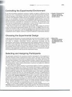
> Exhibit 20-11 Concept Cards for Conjoint Sunglasses Study

C C

Card 2
Watersport Eyewear Comparison
Style 'and design:
Brand name:
Flotation?
Price:

C
Bolle
No
$72

Card 1
Watersport Eyewear Comparison
Style and Design:
Brand Name:
Flotation?
Price:

A
Oakley Eyeshade

Yes

$60

Style and Design

Umited

Multiple color choice: frames, lenses, temples

If brand and price remain unchanged, a design that uses a hard temple with limited color
choices (style C) and no flotation would produce a considerably lower total utility score for
this respondent. For example:

(Style C) - 2.04 + (Oakley brand) 1.31 + (no float) 10.38
• + (price @ $40) 5.90 + (constant) - 8.21 = 7.34
We could also calculate other combinations that would reveal the range of this individual's preferences. Our prediction that respondents would prefer less expensive prices did
not hold for the eighth respondent, as revealed by the asterisk next to the price factor in

_:::EilEZz:lI_K:II...._l:m_:ElIEK;EI~KlICIlIDI!'E

~

_ _. .;TTT.,.

'f,

n~

TTT l f lTl l ' :

T : -; ,


>chapter 20

589

Multivanate Analysis: An Overview

> Exhibit 20-12 Conjoint Results for Participant 8, Sunglasses Study
Subject name: 8
Importance

Utility (s.e.)

-1.4167( .3143)
3.4583( .3685)
-2.0417( .3685)

23.86

Level'

STYLE

Style and design
A
B
C

BRAND

Brand Name
Bolle
Hobbies
Oakley
Ski Optiks

-1.4375( .4083)
.3125( .4083)
1.3125( .4083)
-.1875( .4083)

FLOAT
10.3750( .4715)
20.7500( .9429)
B = 10.3750( .4715)

Flotation?
No
---Yes

PRICE
19.20

1.4750( .2108)
2.9500( .4217)
4.4250( .6325)
5.9000( .8434)

B = 1.4750( .2108)
-8.2083( .9163)

=
=

Price'
$100
$72
$60
$40

CONSTANT

.994
.990 for 4 holdouts

Significance
Significance

=

=

.0000
.0051

.967
1.000 for 4 holdouts

Significance
Significance

=
=

.0000
.0208

Pearson's r
Pearson's r
Kendall's tau
Kendall's tau

'.

Factor

'Subject reversed decision once.

Exhibit 20-12. She reversed herself once on price to get flotation. Other subjects also reversed once on price to trade off for other factors.
The results for the sample are presented in Exhibit 20-13. In contrast to individuals, the
sample placed price first in importance, followed by flotation, style, and brand. Group utilities may be calculated just as we did for the individual. At the bottom of the printout we
find Pearson's r and Kendall's tau. Each was discussed in Chapter 19. In this application,
they measure the relationship between observed and estimated preferences. Since holdout
samples (in conjoint, regression, discriminant, and other methods) are not used to construct
the estimating equation, the coefficients for the holdouts are often a more realistic index of
the model's fit.
Conjoint analysis is an effective tool used by researchers to match preferences to known
characteristics of market segments and design or target a product accordingly. See your student CD for a MindWriter example of conjoint analysis using Simalto+ Plus.

--I!IJ[DbD:LIU:Dl[I1[TITf I:" "11


590

>part IV

Analysis and Presentation of Data

> Exhibit 20-13 Conjoint Results for Sunglasses Study Sample (n = 10)

Importance

18.31

Utility

Factor

Level

STYLE

Style and design
A
B
C

BRAND

Brand Name
Bolle
Hobbies
Oakley
Ski Optiks

FLOAT

----

Flotation?
No
Yes

----

Price
$100
$72
$60
$40

1.1583
-1.9667
.8083

.1938
-.7813
.5187

.0688

5.3875
10.7750
B = 5.3875

PRICE

2.4175
4.8350
7.2525
9.6700
B = 2.4175
-3.4583
Pearson's r
Pearson's r
Kendall's tau
Kendall's tau

;

CONSTANT

.995
.976 for 4 holdouts

Significance
Significance

=

=

.0000
.0120

.950
1.000 for 4 holdouts

Significance
Significance

=
=

.0000
.0208

> Interdependency Techniques
Factor Analysis
Factor analysis is a general term for several specific computational techniques. All have
the objective of reducing to a manageable number many variables that belong together and
have overlapping measurement characteristics. The predictor-criterion relationship that was
found in the dependence situation is replaced by a matrix of intercorrelations among several variables, none of which is viewed as being dependent on another. For example, one
may have data on 100 employees with scores on six attitude scale items.

Method
Factor analysis begins with the construction of a new set of variables based on the relationships in the correlation matrix. While this can be done in a number of ways, the most
frequently used approach is principal components analysis. This method transforms a
set of variables into a new set of composite variables or principal components that are not

""""!El!J~_~-=a:;;I]IX:IIiJISl

n ll-JrT!iJ!!rtlTill"1 TTTTT1 -.--r

!

r } r'-


>chapter 20

591

Mullivar'iate Analysis: An Overview

The world's postal system is projected to grow at a rate of 3.8

groups, and immigranUexpatriate communities. SuperLetter will

percent through 2005, according to its governing body, the

also draw from the $100 billion worldwide international courier

Universal Postal Union (UPU). Hybrid mail will account for 6 per-

. market, like FedEx, UPS, and DHL, now experiencing strong

cent, or 33 billion, of the world's 550 billion pieces of physical

growth rates (15 percent in international volumes relative to single-

mail in 2005 according to the UPU. Superletter.com plans to be

digit domestic growth). But the greatest source of messaging is

an e-business success story in this hybrid-mail sector. According

likely to come from the Internet itself. Focused primarily on inter-

to founder and successful entrepreneur Christopher Schultheiss,

national correspondence, SuperLetter bridges the gap between

"We are establishing the world's first global 'hybrid mail' network

conventional door-to-door postal services, which take from 5 to

enabling users to create letters or documents on their personal

10 days for overseas delivery, and private express/courier ser-

computers, send them like email in a secure encrypted mode

vices, which may take from 2 to 3 days. SuperLetter's basic inter-

over the Internet to remote printers near the recipients, where

national service delivers a letter from desk to door in 2 to 3 days

they will be printed, folded, enveloped, franked with postage and

for about one-tenth of private express costs and under one-half of

delivered in the local mail."

those costs for same-day services.

Using a variety of multiple-variable analytic techniques, Super-

www.superletter.com

Letter specifically identified its target market as professional and
financial service firms, not-for-profit organizations, educational

correlated with each other. These linear combinations of variables, called factors, account
for the variance in the data as a whole. The best combination makes up the first principal
component and is the first factor. The second principal component is defined as the best
linear combination of variables for explaining the variance not accounted for by the first
factor. In tum, there may be a third, fourth, and kth component, each being the best linear
combination of variables not accounted for by the previous factors.
The process continues until all the variance is accounted for, but as a practical matter it
is usually stopped after a small number of factors have been extracted. The output of a principal components analysis might look like the hypothetical data shown in Exhibit 20-14.
Numerical results from a factor study are shown in Exhibit 20-15. The values in this
table are correlation coefficients between the factor and the variables (.70 is the r between
variable A and factor I). These correlation coefficients are called loadings. Two other elements in Exhibit 20-15 need explanation. Eigenvalues are the sum of the variances of the
factor values (for factor I the eigenvalue is .702 + .602 + .502 + .602 + .602 ). When divided
by the number of variables, an eigenvalue yields an estimate of the amount of total variance
explained by the factor. For example, factor I accounts for 36 perceI}t of the total variance.
> Exhibit 20-14 Principal Components Analysis from a Three-Variable Data Set
Component 2

Component 1

Component no. 1

63%

63%

Component no. 2

29

92

Component no. 3

8

100

Component 3

I~Tllf~Jl'lfllllIJ'J1IJJJlJI
III

11


592

>part IV

1

Analysis and F'ros8nlalloll of Uala

> Exhibit 20-15 Factor Matrices

A
Unrotated Factors

Variable

--------I
II
h2

B
Rotated Factors

-----I

II

A

0.70

-.40

0.65

0.79

0.15

B

0.60

-.50

0.61

0.75

0.03

C

0.60

-.35

0.48

0.68

0.10

0

0.50

0.50

0.50

0.06

0.70

E

0.60

0.50

0.61

0.13

0.77

F

0.60

0.60

0.72

om

0.85

Eigenvalue

2.18

1.39

Percent of variance

36.3

23.2

Cumulative percent

36.3

59.5

If a factor has a low eigenvalue, then it adds little to the explanation of variances in the
variables and may be disregarded. The column headed "h 2" gives the communalities, or
estimates of the variance in each variable that is explained by the two factors. With variable A, for example, the communality is .702 + (- AO? = .65, indicating that 65 percent of
the variance in variable A is statistically explained in terms of factors I and II.
In this case, the unrotated factor loadings are not informative. What one would like to

find is some pattern in which factor I would be heavily loaded (have a high r) on some variables and factor II on others. Such a condition would suggest rather "pure" constructs underlying each factor. You attempt to secure this less ambiguous condition between factors
and variables by rotation. This procedure allows choices between orthogonal and oblique
methods. (When the factors are intentionally rotated to result in no correlation between the
factors in the final solution, this procedure is called orthogonal; when the factors are not
manipulated to be zero correlation but may reveal the degree of correlation that exists naturally, it is called oblique.) We illustrate an orthogonal solution here.
To understand the rotation concept, consider that you are dealing only with simple twodimensional rather than multidimensional space. The variables in Exhibit 20-15 can be
plotted in two-dimensional space as shown in Exhibit 20-16. Two axes divide this space,
and the points are positioned relative to these axes. The location of these axes is arbitrary,
and they represent only one of an infinite number of reference frames that could be used to
reproduce the matrix. As long as you, do not change the intersection points and keep the
axes at right angles, when an orthogonal method is used, you can rotate the axes to find a
better solution or position for the reference axes. "Better" in this case means a matrix that
makes the factors as pure as possible (each variable loads onto as few factors as possible).
From the rotation shown in Exhibit 20-16, it can be seen that the solution is improved substantially. Using the rotated solution suggests that the measurements from six scales may
be summarized by two underlying factors (see the rotated factors section of Exhibit 20-15).
The interpretation of factor loadings is largely subjective. There is no way to calculate
the meanings of factors; they are what one sees in them. For this reason, factor analysis is
largely used for exploration. One can detect patterns in latent variables, discover new concepts, and reduce data. Factor analysis is also applied to test hypotheses with confirmatory
models using SEM.

Example
Student grades make an interesting example. The chairperson of Metro U's MBA program
has been reviewing grades for the first-year students and is struck by the patterns in the

-----------KiI...

rlD"T':ll"I'T"rT'T"rT"T'rTT1rT-rrTTrTTTTTT',TTTl

1 1 ! , , I 1 ! Tl TTl IT

n '

: .-----r""":'"
FfTi : . . ]

•


>chapter 20

593

Multivariat() Analysis: An Ovorview

> Exhibit 20-16 Orthogonal Factor Rotations
Unretated
factor \I
J.

1.0
0.8
0.6
0.4
0.2

-1.0 -0.8

-0.6

-0.4

-0.2
-0.2
-0.4
-0.6

Unrotated
factor I

"" 0.2

""

""

0.4

""

""

0.6

0.8

• C

""

1.0

.A

"~ B

""

-0.8

""

""

""

"

Rotated factor I

-1.0

data. His hunch is that distinct types of people are involved in the study of business, and he
decides to gather evidence for this idea.
Suppose a sample of 21 grade reports is chosen for students in the middle of the GPA
range. Three steps are followed:
1. Calculate a correlation matrix between the grades for all pairs of the 10 courses for
which data exist.
2. Factor-analyze the matrix by the principal components method.
3. Select a rotation procedure to clarify the factors and aid in interpretation.
Exhibit 20-17 shows a portion of the correlation matrix. These. data ~epresent correlation

coefficients between the 10 courses. For example, grades secured in VI (Financial
Accounting) correlated rather well (0.56) with grades received in course V2 (Managerial
Accounting). The next best correlation with VI grades is an inverse correlation (- .44) with
grades in V7 (Production).
After the correlation matrix, the extraction of components is shown in Exhibit 20-18.
While the program will produce a table with as many as 10 factors, you choose, in this
case, to stop the process after three factors have been extracted. Several features in this
table are worth noting. Recall that the communalities indicate the amount of variance in
each variable that is being "explained" by th~ factors. Thus, these three factors account for
about 73 percent of the variance in grades in the financial accounting course. It should be
apparent from these communality figures that some of the courses are not explained well
by the factors selected.
The eigenvalue row in Exhibit 20-18 is a measure of the explanatory power of each factor. For example, the eigenvalue for factor 1 is 1.83 and is computed as follows:

1.83

= (.41)2 + (.01)2 + ... + (.25)2
1111''l' 11 '.11111! J J J J J I I I I ! 11

,s_


594

>part IV

Analysis and Presentation of Data

> Exhibit 20-17 Correlation Coefficients, Metro U MBA Study

Variable

V1

Course

Vi

V2

V3

V10

Financial Accounting

1.00

0.56

0.17

-.01

V2

Managerial Accounting

0.56

1.00

-.22

0.06

V3

Finance

0.17

-.22

1.00

0.42

V4

Marketing

-.14

0.05

-.48

-.10

V5

Human Behavior

-.19

-.26

-.05

-.23

V6

Organization Design

-.21

-.00

-.56

-.05

V7

Production

-.44

-.11

-.04

-.08

V8

Probability

0.30

0.06

0.07

-.10

V9

Statistical Inference

-.05

0.06

-.32

0.06

V10

Quantitative Analysis

-.01

0.06

0.42

1.00

> Exhibit 20-18 Factor Matrix Using Principal Factor with Iterations, Metro U
MBA Study

Variable

Course

Factor 1

Factor 2

Factor 3

Communality

V1

Financial Accounting

0.41

0.71

0.23

0.73

V2

Managerial Accounting

0.01

0.53

-.16

0.31

V3

Finance

0.89

-.17

0.37

0.95

V4

Marketing

-.60

0.21

0.30

0.49

V5

Human Behavior

0.02

-.24

-.22

0.11

V6

Organization Design

-.43

-.09

-.36

0.32

V7

Production

-.11

-.58

-.03

0.35

V8

Probability

0.25

0.25

-.31

0.22

V9

Statistical Inference

-.43

0.43

0.50

0.62

V10

Quantitative Analysis

0.25

0.04

0.35

0.19

Eigenvalue

1.83

1.52

0.95

Percent of variance

18.30

15.20

9.50

Cumulative percent

18.30

33.50

43.00

The percent of variance accounted for by each factor in Exhibit 20-18 is computed by dividing eigenvalues by the number of variables. When this is done, one sees that the three
factors account for about 43 percent of the total variance in course grades.
In an effort to further clarify the factors, a varimax (orthogonal) rotation is used to secure the matrix shown in Exhibit 20-19. The largest factor loadings for the three factors are
as follows:
Factor 1

Financial Accounting

Factor 2

Factor 3

0.84

Finance

0.90

Marketing

0.65

Managerial Accounting

0.53

Organization Design

- .56

Statistical Inference

0.79

Production

- .54

r.'"T· ....... :1-;•

.1

~

~

-,

If

T 1 T'I -: .. '1 71 f f 1 I I I I 1 f ' 1

,~


>chapter 20

595

MultlV(;lriate Analysis: An Overviow

> Exhibit 20-19 Varimax Rotated Factor Matrix, Metro U MBA Study

Variable

Course

Factor 1

Factor 2

Factor 3
J.

V1

Financial Accounting

0.84

0.16

-.06

V2

Managerial Accounting

0.53

-.10

0.14

V3

Finance

-.01

0.90

-.37

V4

Marketing

-.11

-.24

0.65

V5

Human Behavior

-.13

,,-14

-.27

V6

Organization Design

-.08

-.56

-.02

V7

Production

-.54

-.11

-.22

V8

Probability

0.41

-.02

-.24

V9

Statistical Inference

0.07

0.02

0.79

V10

Quantitative Analysis

-.02

0.42

0.09

Interpretation
The varimax rotation appears to clarify the relationship among course grades, but as
pointed out earlier, the interpretation of the results is largely subjective. We might interpret
the above results as showing three kinds of students, classified as the accounting, finance,
and marketing types.
A number of problems affect the interpretation of these results. Among the major ones
are these:
I. The sample is small and any attempt at replication might produce a different pattern
of factor loadings.
2. From the same data, another number of factors rather than three can result in different patterns.
3. Even if the findings are replicated, the differences may be due to the varying .influence of professors or the way they teach the courses rather than to the subject content.
4. The labels may not truly reflect the latent construct that underlies any factors we
extract.
This suggests that factor analysis can be a demanding tool to use. It is powerful, but the results must be interpreted with great care.

Cluster Analysis
Unlike techniques for analyzing the relationships between variables, cluster analysis is a
set of techniques for grouping similar objects or people. Originally developed as a classification device for taxonomy, its use has spread because of classification work in medicine,
biology, and other sciences. Its visibility in those fields and the availability of high-speed
computers to carry out the extensive calculations have sped its adoption in business.
Understanding one's market very often involwes classifying, or "segmenting," customers
into homogeneous groups that have common buying characteristics or behave in similar
ways. Such segments frequently share similar psychological, demographic, lifestyle, age,
financial, or other characteristics.
Cluster analysis offers a means for segmentation research and other business problems
where the goal is to classify similar groups. It shares some similarities with factor analysis,
especially when filctor amilysis is applied to people (Q-analysis) instead of to variables. It
differs from discriminant analysis in that discriminant analysis begins with a well-defined


596

>part IV

Analysis and Presentatlol I of Data

group composed of two or more distinct sets of characteristics in search of a set of variables
to separate them. Cluster analysis starts with an undifferentiated group of people, events,
or objects and attempts to reorganize them into homogeneous subgroups.
'.

Method
Five steps are basic to the application of most cluster studies:

1. Selection of the sample to be clustered (e.g., buyers, medical patients, inventory,

products, employees).
2. Definition of the variables on which to measure the objects, events, or people (e.g.,
market segment characteristics, product competition definitions, financial status,
political affiliation, symptom classes, productivity attributes).
3. Computation of similarities among the entities through correlation, Euclidean distances, and other techniques.
4. Selection of mutually exclusive clusters (maximization of within-cluster similarity
and between-cluster differences) or hierarchically arranged clusters.
5. Cluster comparison and validation.
Different clustering methods can and do produce different solutions. It is important to
have enough information about the data to know when the derived groups are real and not
merely imposed on the data by the method.
The example in Exhibit 20-20 shows a cluster analysis of individuals based on three dimensions: age, income, and family size. Cluster analysis could be used to segment the carbuying population into distinct markets. For example, cluster A might be targeted as
potential minivan or sport-utility vehicle buyers. The market segment represented by cluster B might be a sports and performance car segment. Clusters C and D could both be targeted as buyers of sedans, but the C cluster might be the luxury buyer. This form of
clustering or a hierarchical arrangement of the clusters may be used to plan marketing campaigns and develop strategies.

Example
The entertainment industry.js a complex business. A huge number of films are released
each year internationally with some notable financial surprises. Paris offers one of the
world's best selections of films and sources of critical review for predicting an international
audience's acceptance. Residents of New York and Los Angeles are often surprised to dis> Exhibit 20-20 Cluster Analysis 0(1 Three Dimensions
Income

•
A

•
•

Family size

Age


chapter 20

507

Multiv31'iatn AI1;Jlysis: An Ovnlvi0w

> Exhibit 20-21 Film, Country, Genre, and Cluster Membership
Number of Clusters

---------------Film

Country

Genre

Case

Cyrano de Bergerac

France

DramaCom

/I y a des Jours

France

DramaCom

4
5

5

4

3

2

Nikita

France

DramaCom

Les Noces de Papier

Canada

DramaCom

6

Leningrad Cowboys, , ,

Finland

Comedy

19

2

2

2

2

Storia de Ragazzi . , .

Italy

Comedy

13

2

2

2

2

Conte de Printemps

France

Comedy

2

2

2

2

2

Tatie Danielle

France

Comedy

3

2

2

2

2

Crimes and Misdem , , .

USA

DramaCom

7

3

3

3

2

Driving Miss Daisy

USA

DramaCom

9

3

3

3

2

La Voce della Luna

Italy

DramaCom

12

,3

3

3

2

CheHora E

Italy

DramaCom

14

3

3

3

2

Attache-Moi

Spain

DramaCom

15

3

3

3

2

White Hunter Black. ' ,

USA

PsyDrama

10

4

4

3

2

Music Box

USA

PsyDrama

8

4

4

3

2

Dead Poets Society

USA

PsyDrama

11

4

4

3

2

La Fille aux All . ..

Finland

PsyDrama

18

4

4

3

2

Alexandrie, Encore. , ,

Egypt

DramaCom

16

5

3

3

2

Dreams

Japan

DramaCom

17

5

3

3

2

cover their cities are eclipsed by Paris's average of 300 films per week shown in over 100
locations.
We selected ratings from 12 cinema reviewers using sources ranging from Le Monde to

international publications sold in Paris. The reviews reputedly influence box-office receipts, and the entertainment business takes them seriously.
The object of this cluster example was to classify 19 films into homogeneous subgroups. The production companies were American, Canadian, French, Italian, Spanish,
Finnish, Egyptian, and Japanese. Three gemes of film were represented: comedy, dramatic
comedy, and psychological drama. Exhibit 20-21 shows the data by firm name, country of
origin, and genre. The table also lists the clusters for each film using the average linkage
method. This approach considers distances between all possible pairs rather than just the
nearest or farthest neighbor.
The sequential development of the clusters and their relative distances are displayed in
a diagram called a dendogram. Exhibit 20-22 shows that the clustering procedure begins
with 19 films and continues until all the films are again an undifferentiated group. The solid
vertical line shows the point at which the clustering solution best represents the data. This
determination was guided by coefficients provided by the SPSS program for each stage of
the procedure. Five clusters explain this data ~et.
The first cluster shown in Exhibit 20-22 has three French-language films and one
Canadian film, all of which are dramatic comedies. Cluster 2 consists of comedy films.
Two French and two other European films joined at the first stage, and then these two
groups came together at the second stage. Cluster 3, composed of dramatic comedies, is
otherwise diverse. It is made up of two American films with two Italian films adding to the
group at the fourth stage. Late in the clustering process, cluster 3 is completed when a

f

J' f If f 1111 TT1111111 I i1 f f !! 1l ! f

~

1~ 1r 1J


598

>part IV

Analysi~; ,JIld

Pres(mtLltioli of DatCl

> Exhibit 20-22 Dendogram of Film Study Using Average Linkage Method
Rescaled Distance Cluster Combine
CASE
Label
A
Hunter
A
Circle
A
Music
Fd
Fille
E
Alexan
J
Dreams
I
Luna
I
Hora
A
Crimes
A

Daisy
S
Attach
F
Conte
F
Tatie
I
Storia
Cowboy Fd
F
Cyrano
F
Nikita
C
Papier
F
Jours

Seq
PO
PO
PO
PO
DC
DC
DC
DC
DC
DC

DC

C
C
C
C
DC
DC
DC
DC

o
5
10
15
20
25
+--------+--------+----t---~--------~--------;

10
11
8
18
16
17
12
14
7
9

15
2
3
13
19
1

5
6
4

Spanish film is appended. In cluster 4, we find three American psychological dramas combined with a Finnish film at the second stage. In cluster 5, two very different dramatic
comedies are joined in the third stage.
Cluster analysis classified these productions based on reviewers' ratings. The similarities
and distances are influenced by flim genre and culture (as defined by the translated language).

Multidimensional Scaling
Multidimensional scaling (MDS) creates a special description of a respondent's perception about a product, service, or other object of interest on a perceptual map. This often
helps the researcher to understand difficult-to-measure constructs such as product quality
or desirability. In contrast to variables that can he measured directly, many constructs are
perceived and cognitively mapped in different ways by individuals. With MOS, items that
are perceived to be similar will fall close together on the perceptual map, and items that are
perceived to be dissimilar will be'farther apart.

Method
We may think of three types of attribute space, each representing a multidimensional map.
First, there is objective space, in which an object can be positioned in terms of its measurable attributes: its flavor, weight, and nutritional value. Second, there is subjective
space, where perceptions ot'the object's flavor, weight, and nutritional value may be positioned. Obje<;;tive and subjective attribute assessments may coincide, but often they do
not. A comparison of the two allows us to judge how accurately an object is being perceived. Individuals may hold different perceptions of an object simultaneously, and these
may be averaged to present a summary measure of perceptions. In addition, a person's

perceptions may vary over time and in different circumstances; such measurements are
valuable to gauge the impact of various perception-affecting actions, such as advertising
programs.

r

nTTTTT1JTTTTTllTrTrr1

11

j

j'


,;,chapter 20

599

Multivariate AnalysIs: An Ovorview

> Exhibit 20-23 Similarities Matrix of 16 Restaurants
3
1
2
3
4
5
b

f
&
9

10
11
12
13
14
15
1b

4

5

6

7

II

9

10

11

12

13

14

15

16

0

II. 7

0
111.5 15.2
0
4.9 111.7
0.2
0
4.1 3.7 1'1.5 4.3
0
.a.5 4.0 n.1l 11.7 5.8
0
1.1 5.3 111.3 1.2 3.11 11.9
0
8.5
4.1 15.3 11.6 7.6 3.9 9.3
0
4.7 5.9 21.1
4.5 7.8 9.7 5.7 7.7
0

6.9 5.5 1J..8 7.1 2.8 5.5 b.5 /l.5 10.5
0
3.7 7.2 22.0 3.5 7.8 11.2 '1.5 10.0 2.9 10.6
0
0
11.2 10.6 25.11 11.1 12.1 14.4 9.1 12.0 4.7 14.9 4.6
23.11 21.0 6.2 24.0 19.7 17.11 23.4 21.5 26.9 16.9 27.4 31.5
0
lLO 16.5
2.1
2.3 2.0 7.2 1.9 11.0 b.3 4.11 5.11 10.3 21.7

0

With a third map we can describe respondents' preferences using the object's attributes.
This represents their ideal; all objects close to this ideal point are interpreted as preferred
by respondents to those that are more distant Ideal points from many people can be positioned in this preference space to reveal the pattern and size of preference clusters, These
can be compared to the subjective space to assess how well the preferences correspond to
perception clusters. In this way, cluster analysis and MDS can be combined to map market
segments and then examine products designed for those segments.

Example
We illustrate multidimensional scaling with a study of 16 restaurants in a resort area. II The
restaurants chosen represent medium-price family restaurants to high-price gourmet restaurants. We created a metric algorithm measuring the similarities among the 16 restaurants by
asking patrons questions on a 5-point metric scale about different dimensions of service
quality and price. The matrix of similarities is shown in Exhibit 20-23. Higher numbers reflect the items that are more dissimilar.
We might also ask participants to judge the similarities between all possible pairs of
restaurants; then we produce a matrix of similarities using (nonmetric) ordinal data. The
matrix would contain ranks with 1 representing the most similar pair and n indicating the
most dissimilar pair.

A computer program is used to analyze the data matrix and generate a perceptual map.12
The objective is to find a multidimensional spatial pattern that best reproduces the original
order of the data. For example, the most similar pair (restaurants 3, 6) must be located in
this multidimensional space closer together than any other pair. The least similar pair·
(restaurants 14, 15) must be the farthest apart. The computer program presents these relationships as a geometric configuration so that all distances between pairs of points closely
correspond to the original matrix.
Determining how many dimensions to use is complex. The more dimensions of space
we use, the more likely the results will closely match the input data. Any set of n points can
be satisfied by a configuration of n - 1 dimensions. Our aim, however, is to secure a structure that provides a good fit for the data and has the fewest dimensions. MDS is best understood using two or at most three dimensions.
Most software programs include the. calculation of a stress index (S-stress or
Kruskal's stress) that ranges from the worst fit (l) to the perfect fit (0). This study, for
example, had a stress of .001. Another index, R2, is interpreted as the proportion of variance of transformed data accounted for by distances in the model. A result close to 1.0 is
desirable.
In the restaurants example, we conclude that two dimensions represent an acceptable
geometric configuration, as shown in Exhibit 20-24. The distance between Crab Pot and

•.

,

I


600

>part IV

Analysis and Presentation of Data

> Exhibit 20-24 Positioning of Selected Restaurants

High on price

,.
4

Jordan's +
Bistro Z
+

2

o

Chophouse
Ruth; Chris + Flagler Grill
Chuck and Harold'S-----.+
Marc's
+
Tokyo Japanese

Dolphin Bar +

D~'1

Crab Pot

-2

I-

Bones BBQ

+
Thai
Breezes

High on service quality

Key Grill

+ Chinese Buffet
+ Ramirez Mexican

-4
-1.5

-1

-0.5

o

0.5

1.5

Bones BBQ (3, 6) is the shortest, while that between Ramirez Mexican and Jordan's (14,
15) is the longest. As with factor analysis, there is no statistical solution to the definition of
the dimensions represented by the X and Yaxes. The labeling is judgmental and depends on
the insight of the researcher, analysis of information collected from respondents, or another

basis. Respondents sometimes are asked to state the criteria they used for judging the similarities, or they are asked to judge a specific set of criteria.
Consistent with raw data, Jordan's and Bistro Z have high price but service quality close
to the sample mean. In contrast, Flagler and Key Grills generated a price close to the sample's average while providing higher service quality. We could hypothesize that the latter
two restaurants may be run more efficiently-are smaller and less complex-but that
would need to be confirmed with another study. The clustering of companies in attribute
space shows that they are perceived to be similar along the dimensions measured.
MDS is most often used to assess perceived similarities and differences among objects.
Using MDS allows the researcher to understand constructs that are not directly measurable.
The process provides a spatial map thau;hows similarities in terms of relative distances. It is
best understood when limited to two or three dimensions that can be graphically displayed.

1 Multivariate techniques are classified into two categories: dependency and interdependency. When a problem reveals the
presence of criterion and predictor variables, we .have an assumption of dependence. If the variables are interrelated
without designating some as dependent and others independent, then interdependence of the variables is assumed.
The choice of techniques is guided by the number of dependent and independent variables involved and whether they
are measured on metric or nonmetric scales.

2 Multiple regression is an extension of bivariate linear regression. When a researcher is interested in explaining or predicting a metric dependent variable from a set of metric
independent variables (although dummy variables may also
be used), multiple regression is often selected. Regression
results provide information on the statistical significance of
the independent variables, the strength of association between one or more of the predictors and the criterion, and a
predictive equation for future use.


~,chapter

20

Mliltiv;:lriat(J Analysis: An OvcrviRw

H01

researcher to determine the importance of product or ser-

3 Discriminant analysis is used to classify people or objects
into groups based on several predictor variables. The groups

vice attributes and the levels or features that are most desir-

are defined by a categorical variable with two or more val-

able. Respondents provide preference data by ranking or

ues, w~lereas the predictors are metric. The effectiveness of
the discriminant equation is based not only on its statistical

rating cards that describe products. These data become utility weights of product characteristics by means elf optimal

significance but also on its success in correctly classifying

scaling and loglinear algorithms.

cases to groups.

7 Principal components analysis extracts uncorrelated factors

4 Multivariate analysis of variance, or MANOVA, is one of the

. that account for the largest portion of variance from an initial

more adaptive techniques for multivariate data. MANOVA

set of variables. Factor analysis also attempts to reduce the

assesses the relationship between two or more metric

number of variables and discover the underlying constructs

dependent variables and classificatory variables or factors.

that explain the variance. A correlation matrix is used to de-

MANOVA is most commonly used to test differences among
samples of people or objects. In contrast to ANOVA,

rive a factor matrix from which the best linear combination of
variables may be extracted. In many applications, the factor
matrix will be rotated to simplify the factor structure.

MANOVA handles multiple dependent variables, thereby
simultaneously testing all the variables and their

8 Unlike techniques for analyzing the relationships between

interrelationships.

variables, cluster analysis is a set of techniques for grouping
similar objects or people. The cluster procedure starts with

5 Researchers have relied increasingly on structural equation

an undifferentiated group of people, events, or objects and

modeling (SEM) to test hypotheses about the dimensionality
of, and relationships among, latent and observed variables.
Researchers refer to structural equation models as L1SREL

attempts to reorganize them into homogeneous subgroups.
9 Multidimensional scaling (MDS) is often used in conjunction

(linear structural relations) models. The major advantages of

with cluster analysis or conjoint analysis. It allows a respon-

SEM are (1) that multiple and interrelated dependence relationships can be estimated simultaneously and (2) that it

dent's perception about a product, service, or other object of
attitude to be described in a spatial manner. MDS helps the

can represent unobserved concepts, or latent variables, in

business researcher to understand difficult-to-measure con-

these relationships and account for measurement error in

structs such as product quality or desirability, which are per-

the estimation process. Researchers using SEM must follow
five basic steps: (1) model specification, (2) estimation,

ceived and cognitively mapped in different ways by different

(3) evaluation of fit, (4) respecification of the model, and
(5) interpretation and communication.

individuals. Items judged to be similar will fall close together
in multidimensional space and are revealed numerically and
geometrically by spatial maps.

6 Conjoint analysis is a technique that typically handles nonmetric independent variables. Conjoint analysis allows the

average linkage method 597

factors 591

path analysis 575

backward elimination 576

forward selection 576

path diagram 585

beta weights 575

holdout sample 578

principal components analysis 590

centroid 580

interdependency techniques 573

rotation 592

cluster analysis 595

loadings 591

specification error 584

collinearity 577

metric measures 573

standardized coefficients 575

communality 592

multicollinearity 577

stepwise selection 576

conjoint analysis 586

multidimensional scaling (MDS) 598

stress index 599

dependency techniques 573

ml)ltiple regression 574

discriminant analysis 578

multivariate analysis 572

structural equation modeling
(SEM) 583

dummy variable 575

multivariate analysis of variance
(MANOVA) 579

eigenvalue 591
factor analysis 590

utility score 586

nonmetric measures 573

ftflfln TJ n 11 'f III 11' , J J J J ! 1


602

>part IV

Analysis and I'resontation of Data

Terms in Review

1 Distinguish among multidimensional scaling, cluster analysis, and factor analysis.
2 Describe the differences between dependency techniques

graphic data on income levels, ethnicity, and population,
as well as the weather bureau's historical data on temperature. How would you identify geographic areas for
selling dark-colored fabric? You have sample data for

and interdependency techniques. When would you choose

200 randomly selected consumers: their fabric color

a dependency technique?

choice, income, ethnicity, and the average temperature

Making Research Decisions

3 How could discriminant analysis be used to provide insight
into MANOVA results where the MANOVA has one independent variable (a factor with two levels)?
4 Describe how you would create a conjoint analysis study of

of the area where they live.
From Concept to Practice

8 An analyst sought to predict the annual sales for a homefurnishing manufacturer using the following predictor
variables:

= marriages during the year

off-road vehicles. Restrict your brands to three, and suggest possible factors and levels. The full-concept descrip-

Xl

tion should not exceed 256 decision options.

X3 = annual disposable personal income

5 What type of multivariate method do you recommend in

X2 = housing starts during the year
X4 = time trend (first year

each of the following cases and why?
a You want to develop an estimating equation that will be
used to predict which applicants will come to your uni-

= 1, second year = 2, and so

forth)
Using data for 24 years, the analyst calculated the following estimating equation:

versity as students.
b You would like to predict family income using such variables as education and stage in family life cycle..
c You wish to estimate standard labor costs for manufacturing a new dress design.
d You have been studying a group of successful salespeople. You have given them a number of psychological
tests. You want to bring meaning out of these test

results.
6 Sales of a product are influenced by the salesperson's level
of education and gender, as well as consumer income, ethnicity, and wealth.
a Formulate this statement as a multiple regression model
(form only, without parameter estimation).

Y

= 49.85 -

three brands of coffee are influenced by their own income levels and the extent of advertising of the brands.
c Consumer choice of color in fabrics is largely dependent
on ethnicity, income levels, and the temperature of the
geographic area. There is detailed areawide demo-

19.54X4

.92 and a standard

tem of this large county has individuals with purchasing,
service, and maintenance responsibilities. They were asked
to evaluate the vendor/distribution channels of products
that the county purchases. The evaluations were on a 10point metric scale for the following variables:
Delivery speed-amount of time for delivery once the
order has been confirmed.
Price level-level of price charged by the product

price.

b Consumers making a brand choice decision ~between

=

-

9 You are working with a consulting group that has a new
project for the Palm Grove School System. The school sys-

c If the effects of consumer income and wealth are not additive alone, and an interaction is expected, specify a

a Employee job satisfaction (high, normal, low) and employee success (0-2 promotions, 3-5 promotions, 5+
promotions) are to be studied in three different departments of a company.

.036X2 + 1.22X3

The analyst also calculated an R2

suppliers.

7 What multivariate technique would you use to analyze each
of the following problems? Explain your choice.

+

error of estimate of 11.9. Interpret the above equation and
statistics.

b Specify dummy variables.

new variable to test for the interaction.

.068X,

Pri~e

flexibility-perceived willingness to negotiate on

Manufacturer's image-:-manufacturer or supplier's
image.
Overall service-:-Ievel of service necessary to preserve a
satisfactory relationship between buyer and supplier.
Sales force-overall image of the manufacturer's sales
representatives.
Product quality-perceived quality of a particular
product.
The data are found on the text CD.
Your task is to complete an exploratory factor analysis
on the survey data. The purpose for the consulting group is
twofold: (a) to identify the underlying dimensions of these


>chapter 20

data and (b) to create a new set of variables for inclusion
into subsequent assessments of the vendor/distribution
channels. Methodology is.sues to consider in your
analysis are:

603

Over\ll(~w

Multivariato Amllysis: An

b Stay with the new company and give up severance pay.
c Take a transfer to the plant in Chicago.
The researcher gathered data on employee opinions,
inspected personnel files and the like, and

a Desirability of principal components versus principal axis
factoring.

t~en

did a dis-

criminant analysis. Later, when the results were in, she
found the results listed below. How successful was the

b Decisions on criteria for number of factors to extract.

researcher's analysis?

c Rotation of the factors.

Predicted Decision

d Factor loading significance.

Actual Decision

A

e Interpretation of the rotated matrix.

A

80

B
5

12

Prepare a report summarizing your findings and interpreting

B

14

60

14

C

10

15

70

your results.

C

10 A researcher was given the assignment of predicting which
of three actions would be taken by the 280 employees in
the Desota plant that was going to be sold to its employees. The alternatives were to:
a Take severance pay and leave the company.

wwwexerc=ls,.......,e~~~_
FRED II (Federal Reserve Economic Data of the Federal Reserve Bank of St. Louis) is a database of over 1,000 U.S. economic time
series. Visit this Web site ( and select one variable as the dependent variable. What other variables might you use in a multiple regression analysis?

cases*
Mastering Teacher Leadership

NCRCC: Teeing Up and New
Strategic Direction

* Written cases new to this edition and favorite cases from prior editions appear on the text CD; you will find abstracts of these

cases in the Case Abstracts section of this text.

• • • • •!!(;![ITJrITITJ: Tl""TT'f 'r"l>TTl ]"'1 '1 .,

'I 'I 'I , 11 , , , fIT" • • 1 , , I J

!

J

!

!

,

!

!

f

f

,

!

!

I

I

i

I

;

I

I


'.

After reading this chapter, you should understand . ..

1 That a quality presentation of research findings can have an
inordinate effect on a reader's or a listener's perceptions of a study's
quality.
2 The contents, types, lengths, and technical specifications of
research reports.
3 That the writer of a research report should be guided by questions
of purpose, readership, circumstances/limitations, and use.
4 That while some statistical data may be incorporated in the text,
most statistics should be placed in tables, charts, or graphs.
5 That oral presentations of research findings should be developed
with concern for organization, visual aids, and delivery in unique
communication settings. Presentation quality. can enhance or
detract from what might otherwise be excellent research .

. . . . . . .~nmEll'lnmfIni::I'JfTTlFTl'I T I I II I I 1 if 11 fl i , 1 I I 1

I I 1I I

bringingresearchtolife

"Has it occurred to you that your draft of the

"I love the MindWriter project."

MindWriter report has not been touched in the last two

"Ah, there's the problem," she says. "Jason, I have

days? The stack of marked-up pages is right there on

heard you say that you hate projects for other clients,

your desk, and you have been working around it."

and I have heard you say that you like projects. But this

Jason frowns and momentarily flicks his eyes to the
stack of marked pages.

is the first time I have heard you say you love a project.
There comes a time when, after you have nurtured

Sally plunges ahead with her complaint. "It's no big

something, you have to let go. Then it isn't yours. It is

deal, you know. You promised to chop out three pages

someone else's, or it is its own thing, but it is not

of methodology that nobody will care about but your

yours."

fellow statistics jocks ..."-Jason shoots her an ag-

"I guess you're right," Jason smiles sheepishly. ''I'm

grieved look-"... and to remove your recommenda-

a little too invested. This MindWriter project was my

tions and provide them in a separate, informal letter so

baby-well, yours and mine. If I chop three pages out

that Myra Wines can distribute them under her name

of the report, it is finished. Then it belongs to Myra. I

and claim credit for your 'brilliance.'"

don't own it anymore. I can't implement my recom-

"I think I have writer's block."

mendations. I can't change anything. I can't have sec-

"No. Writer's block is when you can't write. You

ond thoughts."

can't unwrite; that's the problem. You have unwriter's

"Fix it, then. Send MindWriter an invoice. Write a

block. Look, some people do great research and then

proposal for follow-up work. Do something, Jason.

panic when they have to decide what goes in the report

Finish it. Let go and move on." Sally smiles and pauses

and what doesn't. Or they can't take all the great ideas

as she is about to leave Jason's office. Jason has pulled

running around in their heads and express their abstrac-

the report to the center of his desk, a very good sign.

tions in words. Or they don't believe they are smart

·"By the way, Custom Foods just called. It awarded

enough to communicate with their clients, or vice

us the contract for its ideation work. I'd hate to work on

versa. So they freeze up. This isn't usually your prob-

that project without you, but ..."

lem. There is some sort of emotional link to this
MindWriter report, Jason; face it."

c

1111 f '1! I till

t, 11111' 111'"

II I 1 I I I I I ~ I I I I I I I I I I

f

I

Itt

I

!

. '

606

-"part IV

Analysis

dll(J

P, eSl:l1latiul1

01

D
> Introduction
As part of the research proposal, the sponsor and the researcher agree on what types of reporting will occur both during and at the end of the research project. Depending-on the budget for the project, a formal oral presentation may not be part of the reporting. A research
sponsor, however, is sure to require a written report. Exhibit 21-1 details the reporting
phase of the research process.

> The Written Research Report
It may seem unscientific and even unfair, but a poor final report or presentation can destroy
a study. Research technicians may ignore the significance of badly reported content, but
most readers will be influenced by the quality of the reporting. This fact should prompt researchers to make special efforts to communicate clearly and fully.
The research report contains findings, analyses of findings, interpretations, conclusions,
and sometimes recommendations. The researcher is the expert on the topic and knows the
specifics in a way no one else can. Because a written research report is an authoritative

> Exhibit 21-1 Sponsor Presentation and the Research Process
Data Analysis & Interpretation

Verbal Data Displays
Tabular Data Displays
Graphical Data Displays
Pictorial Data Displays

FormaVlnformal
Long/Short
TechnicaVMgl.

Discuss and Prepare
Recommendations .

Compile Report/Presentation
-

Deliver Report

-

,

• • • • • • • • • •Dmr2:D:mmD[TllTnrTnTlrTTJ""1lrTT1'Tn·..,I'1fn~r'
..ll"1fl'1r'lrT',.lTTT1Tf nTiTiT'f"1" ;111:-

.


>chapter 21

Presenting Insights and Findings: Written and Oral Reports

one-way communication, it imposes a special obligation for maintaining objectivity. Even
if your findings seem to point to an action, you should demonstrate restraint and caution
when proposing that course.
Reports may be defined by their degree of formality and design. The formal report follows a well-delineated and relatively long format. This is in contrast to the informal or
short report.

Short Reports
Short reports are appropriate when the problem is well defined, is of limited scope, and has
a simple and straightforward methodology. Most informational, progress, and interim reports are of this kind: a report of cost-of-living changes for upcoming labor negotiations or
an exploration of filing "dumping" charges against a foreign competitor.
Short reports are about five pages. If used on a Web site, they may be even shorter. At
the beginning, there should be a brief statement about the authorization for the study, the
problem examined, and its breadth and depth. Next come the conclusions and recommendations, followed by the findings that support them. Section headings should be used.
A letter of transmittal is a vehicle to convey short reports. A five-page reiJort may be
produced to track sales on a quarterly basis. The report should be direct, make ample use
of graphics to show trends, and refer the reader to the research department for further information. Detailed information on the research method would be omitted, although an
overview could appear in an appendix. The purpose of this type of report is to distribute information quickly in an easy-to-use format. Short reports are also produced for clients with
small, relatively inexpensive research projects.
The letter is a form of a short report. Its tone should be informal. The format follows that
of any good business letter and should not exceed a few pages. A letter report is often written in personal style (we, you), although this depends on the situation.
Memorandum reports are another variety and follow the To, From, Subject format.
These suggestions may be helpful for writing short reports:
• Tell the reader why you are writing (it may be in response to a request).
• If the memo is in response to a request for information, remind the reader of the exact point raised, answer it, and follow with any necessary details.
• Write in an expository style with brevity and directness.
• If time permits, write the report today and leave it for review tomorrow before
sending it.

• Attach detailed materials as appendices when needed.

Long Reports
Long reports are of two types, the technical or base report and the management report. The
choice depends on the audience and the researcher's objectives.
Many projects will require both types of reports: a technical report, written for an audience of researchers, and a management report, written for the nontechnically oriented
manager or client. While some researchers try to write a single report that satisfies both
needs, this complicates the task and is seldom satisfactory. The two types of audiences have
different technical training, in"terests, and goals.

The Technical Report
This report should include full documentation and detail. It will normally survive all working papers and original data files and so will become the major source document. It is the

607