Tài liệu Analytical Methods: EViews and Panel Data ppt

Fulbright Economics Teaching Program
First Semester 2002
Analytical Methods
EViews and Panel Data
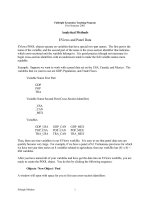
EViews POOL objects operate on variables that have special two-part names. The first part is the
name of the variable, and the second part of the name is the cross-section identifier that indicates
which cross-sectional unit the variable belongs to. It is good practice (though not necessary) to
begin cross-section identifiers with an underscore mark to make the full variable names more
readable.
Example: Suppose we want to work with a panel data set on the USA, Canada, and Mexico. The
variables that we want to use are GDP, Population, and Trade Flows.
Variable Name First Part:
GDP
POP
TRA
Variable Name Second Part (Cross-Section Identifier)
_USA
_CAN
_MEX
Variables
GDP_USA GDP_CAN GDP_MEX
POP_USA POP_CAN POP_MEX
TRA_USA TRA_CAN TRA_MEX
Thus, there are nine variables in our EViews workfile. It is easy to see that panel data sets can
quickly become very large. For example, if we have a panel of 61 Vietnamese provinces for which
we have ten-year time series on 8 variables related to agriculture, then our workfile has (61 x 8) =
488 variables.
After you have named all of your variables and have got the data into an EViews workfile, you are
ready to create the POOL object. You do this by clicking the following sequence:
Objects / New Object / Pool
A window will open with space for you to list your cross-section identifiers:

Eshragh Motahar
1
In the POOL object you refer to variables by the first part name and the question mark. Thus, if
we type a command using GDP? EViews uses all three GDP series for the USA, Canada, and
Mexico.
Notice the button PoolGenr. PoolGenr is used to create new variables according to rules that are
similar to the rules for ordinary Genr. For example, if we want to create GDP Per Capita for all
three countries in our POOL, we would click PoolGenr and then type the equation:
GDPPC? = GDP? / POP?
For estimation, EViews has one
window in which the user specifies
the equation and the assumptions
regarding the stochastic disturbance
term. That window is shown here.
We will describe each element of
the specification window.
Dependent Variable
The dependent variable will be
typed in according to its name and
question mark. For example, you
might use GDPPC?
Eshragh Motahar
2
Sample
By default, EViews will use the largest sample possible in each cross-section. An observation will
be excluded if any of the explanatory or dependent variables for that cross-section are unavailable
in that period.
If the box for Balanced Sample is checked, EViews will eliminate an observation if data are
unavailable for any cross-section in that period.
Common Coefficients

In this field you list all explanatory variables that you assume have the same slope coefficient for
every cross-sectional unit. Use the format VAR? You may use AR(p) specifications if you want
to model autocorrelation. Keep in mind that your panel data set should have a rather long time
series dimension in order to get reliable estimators of the autocorrelation coefficients.
Cross-Section Specific Coefficients
In this window you type the names of all explanatory variables that you assume have different
slope coefficient values for different cross-sectional units. Use the format VAR?
Intercept
Here you specify whether your model has
No intercept ... this case is rare.
Common intercept ... this case is unusual.
Fixed Effects ... the typical specification.
1
Random Effects ... this specification is not often used because it requires strong
assumptions that are difficult to meet in practice.
Weighting
Here, weighting refers to "feasible weighted least squares."
No weighting ... no equation-specific heteroscedasticity.
Cross-section weights ... feasible WLS to correct for equation-specific heteroscedasticity.
SUR ... accounts for contemporaneous cross-equation correlation of errors
and equation-specific heteroscedasticity. To use this, the time-series
dimension must exceed the cross-section dimension (T > N).
1
If you check this option you will see that the EViews output does not report standard errors, t-stats, or p-values for
the estimates of the fixed effects. If you are interested in these (especially for conducting Wald test on these
coefficients), you can enter C in the Cross section specific coefficients edit field, and estimate a
model without a constant; that is, in the Intercept field check None.
Eshragh Motahar
3
Iterate to Convergence ... causes the program to compute new residuals based on the feasible

GLS coefficient estimators, then update the feasible GLS coefficient
estimators; compute new residuals based on the new GLS
coefficient estimators, then update the feasible GLS coefficient
estimators, etc ....
Options
There is only one option: Whites HCCM can be produced if you do not choose SUR.
Hypothesis Testing
In panel data models (as in single-equation multiple-regression models) we are interested in testing
two types of hypotheses: hypotheses about the variances and covariances of the stochastic error
terms and hypotheses about the regression coefficients. The general to simple procedure provides
a good guide.
Before testing hypotheses about the regression coefficients, it is important to have a good
specification of the error covariance matrix so that the test statistics for the regression coefficients
are reliable.
Testing Hypotheses About The Error Covariance Matrix
It is helpful to think about restricted and unrestricted error covariance matrices.
An error covariance matrix is a square matrix with the error variances of the individual cross-
sectional equations along the diagonal and with the contemporaneous error covariances on the off-
diagonal elements. All covariance matrices are symmetric, so if we specify an error covariance
matrix for a panel model with five cross-sectional units we have a (5 x 5) matrix with five diagonal
units and ten off-diagonal units:
2
1 12 13 14 15
2
2 23 24 25
2
3 34 35
2
4 45
2

5





σ σ σ σ σ
σ σ σ σ
σ σ σ
σ σ
σ
If we click the button for SUR, EViews will estimate all of these parameters. On the other hand, if
we believe that the cross-sectional units do not have any contemporaneous cross-equation error
covariances, we would click the button for Cross-Section Weighting and EViews would impose
zero restrictions on all of the off-diagonal elements of the matrix. Only the diagonal elements
would be estimated:
Eshragh Motahar
4
2
1
2
2
2
3
2
4
2
5
0 0 0 0
0 0 0

0 0
0

σ
σ
σ
σ
σ
The second model involves imposing ten restrictions, compared to the first model.
Finally, if we assumed that our stochastic disturbances were free of cross-sectional
heteroscedasticity, we click the No Weighting button and EViews would estimate only one
diagonal element instead of five: four restrictions would be imposed, compared to the second
model.
2
2
2
2
2
0 0 0 0
0 0 0
0 0
0

σ
σ
σ
σ
σ
Testing these restrictions is easily accomplished by means of a test called a likelihood ratio test.
EViews output reports a statistic called the Log-Likelihood. This is an estimator of the joint

probability of the observed sample, given the point estimates of the parameters. As such, it is a
number bounded by zero and one.
All of our estimation methods aim to maximize this log-likelihood. In many applications,
maximizing the log-likelihood leads to exactly the same estimator as the Least-Squares method
does, but the analytical work required is heavier, so we follow the Least-Squares approach.
Our interest here is in the extent to which imposing restrictions on the error covariance matrix
reduces the log-likelihood statistic.
If we form a ratio of the likelihood of a restricted model
ˆ
R
L
divided by the likelihood of an
unrestricted model
ˆ
U
L
, we expect the ratio to be less than 1 because the maximum likelihood
subject to a restriction can be no greater than the maximum likelihood of the unrestricted model.
Define the likelihood ratio:
ˆ

ˆ
R
U
L
L
=l
. Then
0 1
≤ ≤

l
If the restricted model is not significantly different from the unrestricted model we expect the
likelihood ratio to be close to 1. The distribution theory of the likelihood ratio is a bit
cumbersome. However, it is well known that the distribution of
2 log( )− × l
is asymptotically
Chi-Square, so that in any application with a sufficiently large sample size we can use:
Eshragh Motahar
5