Tài liệu Fundament Electric Counter ppt
Bạn đang xem bản rút gọn của tài liệu. Xem và tải ngay bản đầy đủ của tài liệu tại đây (220.81 KB, 44 trang )
1
Application Note 200
Electronic Counter Series
H
Fundamentals of the
Electronic Counters
Time Base
Oscillator
Input Signal
Input Conditioning
Main
Gate
Frequency
Counted
Main Gate
Flip-Flop
Time Base
Dividers
Counting
Register
Display
This literature was published years prior to the establishment of Agilent Technologies as a company independent from Hewlett-Packard
and describes products or services now available through Agilent. It may also refer to products/services no longer supported by Agilent.
We regret any inconvenience caused by obsolete information. For the latest information on Agilent’s test and measurement products go to:
www.agilent.com/find/products
Or in the US, call Agilent Technologies at 1-800-452-4844 (8am–8pm EST)
2
Introduction
Purpose of This Application Note
When Hewlett-Packard introduced its first digital electronic counter, the HP 524A in 1952, a
milestone was considered to have been laid in the field of electronic instrumentation. Frequency
measurement of up to 10 MHz or a 100-ns resolution of time between two electrical events became
possible. Since then, electronic counters have become increasingly powerful and versatile in the
measurements they perform and have found widespread applications in the laboratories, produc-
tion lines and service centers of the telecommunications, electronics, electronic components,
aerospace, military, computer, education and other industries. The advent of the integrated circuit,
the high speed MOS and LSI devices, and lately the microprocessor, has brought about a prolifera-
tion of products to the counter market.
This application note is aimed at introducing to the reader the basic concepts, techniques and the
underlying principles that constitute the common denominator of this myriad of counter products.
Scope
The application note begins with a discussion on the fundamentals of the conventional counter,
the types of measurements it can perform and the important considerations that can have signifi-
cant impact on measurement accuracy and performance. Following the section on the fundamen-
tals of conventional counters comes a section which focuses on counters that use the reciprocal
technique. Then come sections which discuss time interval counters and microwave counters.
Table of Contents
Fundamentals of the Conventional Counters ........................................................................................... 3
The Reciprocal Counters........................................................................................................................... 20
Time Interval Measurement ...................................................................................................................... 24
Automatic Microwave Frequency Counters ........................................................................................... 35
3
Fundamentals of the Conventional Counters
The conventional counter is a digital electronic device which measures the frequency of an input
signal. It may also have been designed to perform related basic measurements including the period
of the input signal, ratio of the frequency of two input signals, time interval between two events
and totalizing a specific group of events.
Functions of the Conventional Counter
Frequency Measurement
The frequency, f, of repetitive signals may be defined by the number of cycles of that signal per
unit of time. It may be represented by the equation:
f =
n
/ t (1)
where n is the number of cycles of the repetitive signal that occurs in time interval, t.
If t = 1 second, then the frequency is expressed as n cycles per second or n Hertz.
As suggested by equation (1), the frequency, f, of a repetitive signal is measured by the conven-
tional counter by counting the number of cycles, n, and dividing it by the time interval, t. The basic
block diagram of the counter in its frequency mode of measurement is shown in Figure 1.
Time Base
Oscillator
Input Signal
Input Conditioning
Main
Gate
Frequency
Counted
Main Gate
Flip-Flop
Time Base
Dividers
Counting
Register
Display
Figure 1. Basic block diagram of the conventional counter in its frequency mode of measurement.
The input signal is initially conditioned to a form that is compatible with the internal circuitry of
the counter. The conditioned signal appearing at the door of the main gate is a pulse train where
each pulse corresponds to one cycle or event of the input signal. With the main gate open, pulses
are allowed to pass through and get totalized by the counting register. The time between the
opening to the closing of the main gate or gate time is controlled by the Time Base. From equation
(1), it is apparent that the accuracy of the frequency measurement is dependent on the accuracy in
which t is determined. Consequently, most counters employ crystal oscillators with frequencies
such as 1, 5 or 10 MHz as the basic time base element.
4
The Time Base Divider takes the time base oscillator signal as its input and provides as an output a
pulse train whose frequency is variable in decade steps made selectable by the Gate Time switch.
The time, t, of equation (1) or gate time is determined by the period of the selected pulse train
emanating from the time base dividers. The number of pulses totaled by the counting register for
the selected gate time yields the frequency of the input signal. The frequency counted is displayed
on a visual numerical readout. For example, if the number of pulses totaled by the counting
register is 50,000, and the selected gate time is one second, the frequency of the input signal is
50,000 Hertz.
Period Measurement
The period, P, of an input signal is the inverse of its frequency.
P f
Ptn
=
∴=
1/
/
(2)
The period of a signal is therefore the time taken for the signal to complete one cycle of oscilla-
tion. If the time is measured over several input cycles, then the average period of the repetitive
signal is determined. This is often referred to as multiple period averaging.
The basic block diagram for the conventional counter in its period measurement mode is shown in
Figure 2. In this mode of measurement, the duration over which the main gate is open is controlled
by the frequency of the input signal rather than that of the time base. The Counting Register now
counts the output pulses from the time-base dividers for one cycle or the period of the input signal.
The conditioned input signal may also be divided so that the gate is open for decade steps of the
input signal period rather than for a single period. This is the basis of the multiple period aver-
aging technique.
Period measurement allows more accurate measurement of unknown low-frequency signals
because of increased resolution. For example, a frequency measurement of 100 Hz on a counter
with 8-digit display and a 1-second gate time will be displayed as 00000.100 KHz. A single period
measurement of 100 Hz on the same counter with 10 MHz time base would display 0010000.0 µs.
The resolution is improved 1000 fold.
Figure 2. Basic block diagram of the conventional counter in its period measurement mode.
Time Base
Oscillator
Input
Signal
Input Conditioning
Main
Gate
Frequency
Counted
Main Gate
FF
Time Base
Dividers
Counting
Register
Display
5
Frequency Ratio of Two Input Signals
The ratio of two frequencies is determined by using the lower-frequency signal for gate control
while the higher-frequency signal is counted by the Counting Register, as shown in Figure 3.
Accuracy of the measurement may be improved by using the multiple averaging technique.
Higher Frequency
Input Signal
Lower Frequency
Input Signal
Input Conditioning
Input Conditioning
Main Gate
FF
Time Base
Dividers
Counting Register Display
Main
Gate
Figure 3. Ratio Measurement Mode
Time Interval Measurement
The basic block diagram of the conventional counter in its time interval mode of measurement is
shown in Figure 4. The main gate is now controlled by two independent inputs, the START input,
which opens the gate, and the STOP input which closes it. Clock pulses from the dividers are
accumulated for the time duration for which the gate is open. The accumulated count gives the
time interval between the START event and the STOP event. Sometimes the time interval may be
for signal of different voltage levels such as t
h
shown in Figure 5. The input conditioning circuit
must be able to generate the START pulse at the 0.5V amplitude point, and the STOP pulse at the
1.5V amplitude point.
Input Conditioning
Input Conditioning
Main Gate
FF
Time Base
Dividers
Counting Register
Display
Main
Gate
Start
Stop
Time Base
Oscillator
Open
Close
Figure 4. Time Interval Measurement Mode
Several techniques are currently available to enhance considerably the resolution of the time
interval measurement. These techniques are discussed along with other details in the section
about time interval measurements beginning on page 24.
6
Voltage
Start
Stop
Time
0
V
2V
x
x
t
h
Figure 5. Measurement of time interval, t
h
, by trigger level adjustment.
Totalizing Mode of Measurement
In the totalizing mode of measurement, one of the input channels may be used to count the total
number of a specific group of pulses. The basis block diagram, Figure 6, for this mode of operation
is similar to that of the counter in the frequency mode. The main gate is open until all the pulses
are counted. Another method is to use a third input channel for totalizing all the events. The first
two input channels are used to trigger the START/STOP of the totalizing activity by opening/
closing the main gate.
Time Base
Oscillator
Input Conditioning
Main
Gate
Main Gate
FF
Time Base
Dividers
Counting
Register
Display
Start/Stop Totalizing
Figure 6. Totalize Measurement Mode
The START/STOP of the totalizing activity can also be controlled manually by a front panel switch.
In the HP 5345A Electronic Counter totalizing of a group of events in two separate signals is done
by connecting the two input signals to Channel A and B. With the Function switch set at START,
the main gate opens to commence the count accumulation. The totalizing operation is terminated
by turning the function switch to STOP position. The readout on the HP 5345A will display either
(A + B) or (A – B) depending on the position of the ACCUM MODE START/STOP switch on the
rear panel.
7
Other Functions of a Conventional Counter
There are three other functions which are sometimes employed in the conventional counter.
Counters employed in these functions are known as:
• Normalizing Counters
• Preset Counters
• Prescaled Counters
A. Normalizing Counters
The normalizing counter displays the frequency of the input signal being measured multiplied by a
numerical constant.
If f is the frequency of the input signal, the displayed value, y, is given by
y = a
·
f where a is a numerical constant.
This technique is commonly used in industrial applications for measurement of RPM or flow rate.
The normalizing factor may be set via thumbwheel switches or by a built-in IC memory circuit.
B. Preset Counters
Preset counters provide an electrical output when the display exceeds the number that is preset in
the counter via a means such as thumbwheel switches. The electrical output is normally used for
controlling other equipment in industrial applications. Examples include batch counting and limit
sensing for engine RPM measurements.
C. Prescaled Counters
Besides the input amplifier trigger, two other elements in the counter limit the reliability of fre-
quency measurement at the upper end. These are the speed of the main gate switches and the
counting registers. One technique that is employed which increases the range of the frequency
response without exacting high speed capabilities of the main gate and counting register is simply
to add a prescaler (divider). The prescaler divides the input signal frequency by a factor, N, before
applying the signal to the main gate. This technique is called prescaling. See Figure 7. However, the
main gate has to remain open N times longer in order to accumulate the same number of counts in
the counting register. Therefore, prescaling involves a tradeoff. The frequency response is in-
creased by a factor of N, but so is the measurement time to achieve the same resolution. A slower
and less expensive main gate and counting register can be used, but at the expense of an addi-
tional divider.
Time Base
Oscillator
Input
Conditioning
Main
Gate
Main Gate
Flip-Flop
Time Base
Dividers
Counting
Register
Display
Input
÷
N Prescaler
÷
N
Figure 7. Block Diagram of Prescaling Counters
8
Prescaled 500-MHz counters are typically less expensive than their direct-count counterparts. For
measurement of average frequency, prescaled counters may be satisfactory. However, their limita-
tions include:
• poorer resolution by factor of N for same measurement time
• short measurement times (e.g. 1 µs) are typically not available
• cannot totalize at rates of the upper frequency limits indicated
9
Important Basic Considerations That Affect Performance of
the Conventional Counter
Input Considerations
The major elements of the input circuitry are shown in Figure 8 and consist of attenuator, amplifier
and Schmitt trigger. The Schmitt trigger is necessary to convert the analog output of the input
amplifier into a digital form compatible with the counter’s counting register.
Input
Attenuator
Amplifier
Schmitt Trigger
Figure 8. Major elements of a counter’s input circuitry
A. Sensitivity
The sensitivity of a counter is defined as the minimum specified input signal that can be counted.
Sensitivity is usually specified in terms of the RMS value of a sinusoidal input. For pulse type
inputs, therefore, the minimum pulse amplitude sensitivity is 2 of the specified value of the
trigger level.
The amplifier gain and the voltage difference between the Schmitt trigger hysteresis levels deter-
mine the counter’s sensitivity. At first glance it might be thought that the more sensitive the coun-
ter input, the better. This is not so. Since the conventional counter has a broadband input and with
a highly sensitive front end, noise can cause false triggering. Optimum sensitivity is largely depend-
ent on input impedance, since the higher the impedance the more susceptible to noise and false
counts the counter becomes.
Inasmuch as the input to a counter looks like the input to a Schmitt trigger, it is useful to think of
the separation between the hysteresis levels as the peak-peak sensitivity of the counter. To effect
one count in the counter’s counting register, the input must cross both the upper and lower hyster-
esis levels. This is summarized by Figure 9.
Upper
Hysteresis
Level
Peak-Peak
Sensitivity
Lower
Hysteresis
Level
Output From
Schmitt Trigger
Input Signals
to Counter
OV
(a) (b)
Figure 9. Input Characteristics. To effect a count the signal must cross through both the upper and lower
hysteresis levels. Thus in (b), the “ringing” on the input signal shown does not cause a count.
2
10
B. ac-dc Coupling
As Figure 10 shows, ac coupling of the input is almost always provided to enable signals with a dc
content to be counted.
Upper
Hysteresis
Level
Lower
Hysteresis
Level
(a)
dc Coupling
(b)
ac Coupling
OV
Figure 10. ac-dc Coupling. An input signal with the dc content shown in (a) would not be counted unless ac
coupling, as shown in (b), was used to remove the signal’s dc content.
C. Trigger Level
In the case of pulse inputs, ac coupling is of little value if the duty cycle is low. Moreover, ac
coupling should not be used on variable duty cycle signals since the trigger point varies with duty
cycle and the operator has little idea where his signal levels are in relation to ground at the ampli-
fier input. The function of the trigger level control is to shift the hysteresis levels above or below
ground to enable positive or negative pulse trains respectively, to be counted. This is summarized
in Figure 11.
(c)
(b)
(a)
V
u
V
L
V
c
V
u
V
L
V
c
V
u
V
L
V
c
Figure 11. Trigger Level Control. The signal (a) will not be counted. Using the trigger level control to shift the
hysteresis levels above ground (b), enables a count. For negative pulse trains (c), the hysteresis levels can be
moved below ground.
Many counters provide a three position level control with the “preset” position corresponding to
Figure 11 (a), a position normally labeled “+” corresponding to Figure 11 (b) and “–” for the Figure
11 (c) case. The more sophisticated counters provide a continuously adjustable trigger level
control, adjustable over the whole dynamic range of the input. This more flexible arrangement
ensures that any signal within the dynamic range of the input and of an amplitude consistent with
the counter’s sensitivity can be counted.
11
D. Slope Control
The slope control determines if the Schmitt circuit is triggered by a signal with a positive (+) slope
(going from one voltage level to another of a more positive level regardless of polarity) to generate
an output pulse at the upper hysteresis limit (V
u
) or by a signal with a negative (–) slope which
causes an output pulse to be generated at the lower hysteresis limit (V
L
).
E. Dynamic Range
The dynamic range of the input is defined as the input amplifier’s linear range of operation. Clearly,
it is not important for the input amplifier of a frequency counter to be absolutely linear as it is in
an oscilloscope for example (this is not the case for time interval, see “Time Interval Measure-
ment” on page 24). With a well designed amplifier, exceeding the dynamic range will not cause
false counts. However, input impedance could drop and saturation effects may cause the amplifier
speed of response to decrease. Of course, all amplifiers have a damage level and protection is
usually provided. Conventional protection often fails, however, where high speed transients (e.g.,
at turn-on of a transmitter) and low impedance 50Ω inputs are involved. To this end, several of the
Hewlett-Packard counters (HP 5328A and HP 5305B) employ high speed fuses, in addition to the
conventional protection, to further protect the wideband 50Ω input amplifiers.
F. Attenuators
It is, nevertheless, not good practice to exceed the dynamic range of the input. To avoid this on
larger level signals, attenuators are provided. The more sophisticated inputs with wide dynamic
range usually employ step attenuators with attenuation positions such as X1, X10, and X100.(These
positions represent nominal attenuation. The attenuation values used depend on the dynamic
range of the input.) Another variation is a variable attenuation scheme. This is mandatory for low
dynamic range inputs, but it also provides the additional advantage of variably attenuating noise
signals to minimize the noise while maintaining maximum signal amplitude.
G. Input Impedance
For frequencies up to around 10 MHz, a 1 MΩ input impedance is usually preferred. With this
impedance level, the majority of sources connected to the input are not loaded, and the inherent
shunt capacity of about 35 pF has little effect. As noted earlier, for noise considerations, sensitivi-
ties of 25 mV to 50 mV are preferred. Beyond about 10 MHz, however, the inherent shunt capacity
of high impedance inputs rapidly reduces input impedance. For this reason, 50Ω impedance levels,
which can be provided with low shunt capacity, are preferred. Sensitivities of 10 mV are techno-
logically feasible but because of noise and related problems 20 mV to 25 mV are considered
optimum with 50Ω inputs. A sensitivity of 1 mV, for example, is possible, of course, however the
user must pay a premium for this and noise problems can occur.
H. Automatic Gain Control
Automatic Gain Control (AGC) may be thought of as an automatically adjustable sensitivity
control. The gain of the amplifier-attenuator section of the input (see Figure 8) is automatically set
by the magnitude of the input signal.
A tradeoff exists between the speed of response of the automatic gain control and the minimum
frequency signal that can be counted. For this reason the lower frequency limit for AGC inputs is
usually around 50 Hz. AGC inputs, therefore, are useful primarily for frequency measurements
only.
12
AGC provides a certain amount of operator ease since the sensitivity control is eliminated. A
second advantage of AGC is its ability to handle input signals of time varying amplitude. Figure 12
shows an example of this. The output of a magnetic transducer is shown as the frequency as the
rotating member reduces from 3300 Hz to 500 Hz. The signal level decreases from 800 mV to
200 mV and the noise decreases from 300 mV to 50 mV. If the sensitivity were set to count the
lower level signal, any attempt to count the higher level signal at 3300 Hz would result in false
counts due to the 300 mV noise level. AGC eliminates this problem since the noise shown on the
high level signal is attenuated, along with the signal, to a level where it does not cause false trigger-
ing. This assumes, of course, that the trigger level is appropriately set in the first place.
AGC has limitations in measurement of high frequency signals with AM modulation. Since the AGC
circuit makes adjustments for the measurement near the peak levels and ignores the valleys of the
input signal, erroneous counting can result due to the presence of AM modulation in high fre-
quency signals.
800 mV
300 mV
200 mV
50 mV
(a) (b)
Figure 12. Output of a magnetic transducer at 3300 Hz (a) and 500 Hz (b). Without AGC it would be
impossible to measure this changing frequency since a sensitivity setting to measure the lower frequency signal
would result in erroneous counts due to noise at the higher frequencies.
Figure 13 summarizes the various conditioning of the input signal prior to its application to the
main gate of the counter.
Main
Gate
Amp
Input
Impedance
AGC
Limiter
Fuse
Trigger
Level
Control
Schmitt
Trigger
Trigger
Slope
Atten
Trigger
Light
ac/dc
Coupling
Figure 13. Input Signal Conditioning
13
Time Base Oscillator Considerations
The source of the precise time, t, as defined in equation (1) is the time base oscillator. Any error
inherent in the value of t will be reflected in the accuracy of the counter measurement. In this
section, the different types of time base oscillators used in a counter are reviewed along with the
basic factors that can affect the accuracy of the oscillator. Most counters employ a quartz crystal
as the oscillating element.
A. Types of Time Base Oscillators
The three basic types of crystal oscillators are:
• Room temperature Crystal Oscillator (RTXO)
• Temperature Compensated Crystal Oscillator (TCXO)
• Oven Controlled Crystal Oscillator
The Room Temperature crystal oscillators are those which have been manufactured for minimum
frequency change over a range of temperature — typically between 0°C to 50°C. This is accom-
plished basically through the proper choice of the crystal cut during the manufacturing process. A
high quality RTXO would vary by about 2.5 parts per million over the temperature range of 0°C to
50°C.
The electrical equivalent circuit of the quartz crystal is shown in Figure 14. The values of R
1
, C
1
,
L
1
, and C
0
are determined by the physical properties of the crystal. An external variable
capacitance is typically added to obtain a tuned circuit. The L, C and R are the elements that
make the frequency of the crystal oscillator temperature sensitive. Hence, one obvious method of
compensating for frequency changes due to temperature variation is to control some externally
added capacitance or components with opposite temperature coefficient to obtain a more stable
frequency of the tuned circuit. Oscillators with this method of compensation are often called
Temperature Compensated crystal oscillators (TCXO). These oscillators offer an order of magni-
tude improvement in frequency stability over that of the Room Temperature uncompensated type.
Typical frequency changes are 5 × 10
-7
over 0°C to 50°C temperature range, or five times better
than that of the RTXO.
C
1
L
1
C
0
R
1
Figure 14. Equivalent Circuit of the Crystal
The third type of oscillator used in counters is the Oven Controlled crystal oscillator. In this
technique, the crystal oscillator is housed in an oven which minimizes the temperature changes
surrounding the crystal. Two types of ovens are typically employed — the simple ON/OFF switch-
ing oven and the proportional oven. The simple switching oven turns the power OFF when the
maximum temperature is reached and ON when the minimum temperature is reached. The more
sophisticated proportional oven controls and provides a heating that is proportional to the differ-
ential between the actual temperature and the desired temperature surrounding the crystal
oscillator inside the oven. Typical variation in frequency for a high quality proportional oven
controlled crystal oscillator is less than 7 parts in 10
9
over the 0°C to 50°C temperature range.
14
It usually takes 24 hours or more after turn-on for the oven oscillator to achieve its specified
stability. However, it can come to 5 parts in 10
9
of the final specified frequency value after a 20-
minute warm-up. Most counters employing an oven oscillator have a feature whereby the oscilla-
tor is powered whenever the power line is connected even if the counter is not turned on. Keeping
the counter connected to the power line avoids the need for the warm-up phase and retrace.
B. Factors Affecting Accuracy of Crystal Oscillators
Apart from the temperature effects, there are other significant factors which can affect the accu-
racy of the oscillator frequency. These other factors are Line Voltage Variation, Aging or Long Term
Stability, Short Term Stability, Magnetic Fields, Gravitational Fields and Environmental factors
such as vibration, humidity and shock. The first three factors are the significant ones and are
discussed below.
1. Effect of Line Voltage Variations
Variations in the line voltage causes variations in the oscillator frequency. The amount of variation
in the voltage applied to the oscillator and its associated circuit, of course, would depend on the
effectiveness of any voltage regulator incorporated in the instrument. Changes in the level of the
regulated voltage applied to the oscillator and its associated circuit or the oven controller would
cause changes on bias levels, phase of feedback signal resulting in variation in the output oscilla-
tor frequency. A high stability, Oven Controlled oscillator would provide frequency stability on the
order of 1 part per 10
10
for 10 percent change in the line voltage applied to the oven. For RTXO,
the frequency stability is typically on the order of 1 part per 10
7
for the same 10 percent change in
line voltage. Regulation better than this is unnecessary as frequency variations due to temperature
effects would mask the effects of line voltage changes.
2. Aging Rate or Long Term Stability
The physical properties of the quartz crystal exhibit a gradual change with time resulting in a
gradual cumulative frequency drift called Aging. See Figure 15. The aging rate is dependent on the
inherent quality of the crystals used. Aging goes on all the time. Aging is often specified in terms of
frequency changes per month since temperature and other effects would mask the small amount
Figure 15. Effect of Aging on Frequency Stability
Days from Calibration
Short Term Stability
Long Term Stability or Aging
Parts per 10
9
Change
70
60
50
40
30
20
10
0 5 10 15 20 25
15
of aging for a shorter time period. Aging for air crystals is given in frequency changes per month as
it is not practical to accurately and correctly measure over any shorter averaging period. For a
good RTXO, the aging rate is typically on the order of 3 parts per 10
7
per month. For a high quality
Oven controlled oscillator, the aging rate is typically 1.5 parts per 10
8
per month.
3. Short Term Stability
Often referred to as the Time Domain Stability, or fractional frequency deviation, short term
stability is the result of the inevitable noise (random frequency and phase fluctuations) generated
in the oscillator.
Since this noise is spectrally related, any specification of short term stability must include the
averaging or measurement time involved. The effect of this noise usually varies inversely with
measurement time. With quoted averaging time, the specification of short term stability essentially
specifies the uncertainty due to noise in the oscillator frequency over the quoted time period. The
accepted measure in the time domain is called Allan Variance. In practice, the square root of a
particular Allan Variance is given as
σ
∆f
f
t
()
()
. It is akin to the RMS of the frequency variations
given for different averaging times.
Figure 16 summarizes the oscillator characteristics described, utilizing typical specifications of
well designed oscillators.
Figure 16. Typical specifications of the four types of oscillators
The total time base oscillator error is the cumulative effect of all the individual sources of error
described above. The time base error is only one of the several sources of measurement error for
the counter. Hence, it may or may not be significant for a given counter measurement depending
on the particular application involved. Sources of counter measurement errors are described on
following pages.
Main Gate Requirements
As with any physical gate, the main gate of the counter does exhibit propagation delays and takes
some finite time to both switch ON and OFF. This finite amount of switching time is reflected in
the total amount of time the gate is open for counting. If this switching time is significant com-
pared to the period of the highest frequency counted, errors in the count will result. However, if
this switching time is significantly less compared to the period of the highest frequency counted,
the error is not appreciable. For a 500-MHz signal with 2 ns period, this error will be insignificant if
Room Temperature
Crystal Oscillators
Temperature
Compensated
Crystal Oscillators
Simple Switching
Oven Oscillators
Proportional
Oven Oscillators
Temperature <2.5 × 10
–6
<5 × 10
–7
<1 × 10
–7
<7 × 10
–9
(0°C - 50°C)
Line Voltage <1 × 10
–7
<5 × 10
–8
<1 × 10
–9
<1 × 10
–10
(10% change)
Aging <3 × 10
–7
/mo <1 × 10
–7
/mo <1 × 10
–7
/mo <1.5 × 10
–8
/mo
or
<5 × 10⁻¹⁰ /day
(1 sec avg.)
Short Term <2 × 10
–9
rms <1 × 10
–9
rms <5 × 10
–10
rms <1 × 10
–11
rms
16
the switching time of the main gate is substantially less than 1 ns. For true 500 MHz operation,
high-speed devices are necessary in the gate, input and counting register circuitry. The HP 5345A
Electronic Counter achieves this objective through the use of specially designed emitter-emitter
coupled logic circuits.
Sources of Measurement Error
The major sources of measurement error for an electronic counter are generally classified into the
following four categories:
• the ±1 count error
• the Time Base error
• the Trigger error
• the Systematic error
A. Types of Measurement Error
1. The ±1 Count Error
When an electronic counter makes a measurement, a ±1 count ambiguity can exist in the least
significant digit. This is often referred to as quantization error. This ambiguity can occur because
of the non-coherence between the internal clock frequency and the input signal as illustrated in
Figure 17. The error caused by this ambiguity is, in absolute terms, ±1 out of the total accumulated
count.
t
m
t
m
Signal Input to Main Gate
Gate Opening Case No. 1
Gate Opening Case No. 2
Figure 17. ±1 Count Ambiguity. The main gate is open for the same time t
m
in both cases. Incoherence between
the clock and the input signal can cause two valid counts which for this example are 1 for Case No. 1
and 2 for Case No. 2.
2. The Time Base Error
Any error resulting from the difference between the actual time base oscillator frequency and its
nominal frequency is directly translated into a measurement error. This difference is the cumula-
tive effect of all the individual time base oscillator errors described previously and may be ex-
pressed as dimensionless factor such as so many parts per million.
3. Trigger Error
Trigger error is a random error caused by noise on the input signal and noise from the input
channels of the counter. In period and time interval measurements, the input signal(s) control the
opening and closing of the counter’s gate. The effect of the noise is to cause one limit of the
hysteresis window to be crossed too soon or too late — causing the main gate to be open for an
incorrect period of time. This results in a random timing error for period and time interval
measurements.
17
4. Systematic Error
For time interval measurements, any slight mismatch between the start channel and the stop
channel amplifier risetimes and propagation delays results in internal systematic errors. Mis-
matched probes or cable lengths introduce external systematic errors.
For time interval measurements, trigger level timing error is another systematic error which is
caused by uncertainty in the actual trigger point. This uncertainty is not due to noise, however, but
is due to offsets in trigger level readings caused by hysteresis and drifts. Trigger level timing error
may be expressed as
∆T =
trigger level error
signal slew rate at trigger point
Not all these four categories of measurement error are significant for all modes of counter meas-
urement. As summarized in Figure 18, only the ±1 count and time base errors are considered as
important for frequency measurements using conventional counters.
In period measurement, all of the first three types of error can affect the accuracy of the measure-
ment, while all the four types of error can be significant for time interval measurements.
±1 Count Yes Yes Yes A Random error
± Time Base Yes Yes Yes
± Trigger Yes Yes A Random error
± Systematic Yes
Source of Errors
Frequency
Measurement
Period
Measurement
Time Interval
Measurement
Remarks
Figure 18. Summary of Measurement Errors
B. Frequency Measurement Error
The accuracy of an electronic counter is dependent on the mode of operation.
The total frequency measurement error may be defined as the sum of its ±1 count error and its
total time base error. The relative frequency measurement error due to ±1 count ambiguity is
∆f
ff
in
=
±1
where f
in
is the input signal frequency.
Hence, the higher the signal frequency, the smaller the relative frequency measurement error due
to ±1 count. The relative frequency measurement error due to the time base error is a
dimensionless factor usually expressed in parts per million. If the total error of the time base
amounted to say one part per million (1 × 10
–6
), the error contributed by the time base in the
measurement of a 10-MHz signal is
(1 × 10
–6
) × 10
7
Hz or 10 Hz.
Or, the relative frequency measurement error due to the time base error is ±1 × 10
–6
. And that due
to the ±1 count error is ±1/10
7
or ±1 × 10
–7
for a one second gate.
In this particular example, therefore, the ±1 count error becomes dominant for input frequency
less than 1 MHz but is masked by the time base error for input frequency higher than 1 MHz.