Tài liệu Image and Videl Comoression P2 doc

2

© 2000 by CRC Press LLC

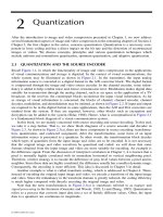
Quantization

After the introduction to image and video compression presented in Chapter 1, we now address
several fundamental aspects of image and video compression in the remaining chapters of Section I.
Chapter 2, the first chapter in the series, concerns quantization. Quantization is a necessary com-
ponent in lossy coding and has a direct impact on the bit rate and the distortion of reconstructed
images or videos. We discuss concepts, principles and various quantization techniques which
include uniform and nonuniform quantization, optimum quantization, and adaptive quantization.

2.1 QUANTIZATION AND THE SOURCE ENCODER

Recall Figure 1.1, in which the functionality of image and video compression in the applications
of visual communications and storage is depicted. In the context of visual communications, the
whole system may be illustrated as shown in Figure 2.1. In the transmitter, the input analog
information source is converted to a digital format in the A/D converter block. The digital format
is compressed through the image and video source encoder. In the channel encoder, some redun-
dancy is added to help combat noise and, hence, transmission error. Modulation makes digital data
suitable for transmission through the analog channel, such as air space in the application of a TV
broadcast. At the receiver, the counterpart blocks reconstruct the input visual information. As far
as storage of visual information is concerned, the blocks of channel, channel encoder, channel
decoder, modulation, and demodulation may be omitted, as shown in Figure 2.2. If input and output
are required to be in the digital format in some applications, then the A/D and D/A converters are
omitted from the system. If they are required, however, other blocks such as encryption and
decryption can be added to the system (Sklar, 1988). Hence, what is conceptualized in Figure 2.1
is a fundamental block diagram of a visual communication system.
In this book, we are mainly concerned with source encoding and source decoding. To this end,

we take it a step further. That is, we show block diagrams of a source encoder and decoder in
Figure 2.3. As shown in Figure 2.3(a), there are three components in source encoding: transforma-
tion, quantization, and codeword assignment. After the transformation, some form of an input
information source is presented to a quantizer. In other words, the transformation block decides
which types of quantities from the input image and video are to be encoded. It is not necessary
that the original image and video waveform be quantized and coded: we will show that some
formats obtained from the input image and video are more suitable for encoding. An example is
the difference signal. From the discussion of interpixel correlation in Chapter 1, it is known that a
pixel is normally highly correlated with its immediate horizontal or vertical neighboring pixel.
Therefore, a better strategy is to encode the difference of gray level values between a pixel and its
neighbor. Since these data are highly correlated, the difference usually has a smaller dynamic range.
Consequently, the encoding is more efficient. This idea is discussed in Chapter 3 in detail.
Another example is what is called transform coding, which is addressed in Chapter 4. There,
instead of encoding the original input image and video, we encode a transform of the input image
and video. Since the redundancy in the transform domain is greatly reduced, the coding efficiency
is much higher compared with directly encoding the original image and video.
Note that the term transformation in Figure 2.3(a) is sometimes referred to as

mapper

and

signal processing

in the literature (Gonzalez and Woods, 1992; Li and Zhang, 1995). Quantization
refers to a process that converts input data into a set of finitely different values. Often, the input
data to a quantizer are continuous in magnitude.

© 2000 by CRC Press LLC

Hence, quantization is essentially discretization in magnitude, which is an important step in
the lossy compression of digital image and video. (The reason that the term lossy compression is
used here will be shown shortly.) The input and output of quantization can be either scalars or
vectors. The quantization with scalar input and output is called

scalar



quantization

, whereas that
with vector input and output is referred to as

vector



quantization

. In this chapter we discuss scalar
quantization. Vector quantization will be addressed in Chapter 9.
After quantization, codewords are assigned to the many finitely different values from the output
of the quantizer. Natural binary code (NBC) and variable-length code (VLC), introduced in
Chapter 1, are two examples of this. Other examples are the widely utilized entropy code (including
Huffman code and arithmetic code), dictionary code, and run-length code (RLC) (frequently used
in facsimile transmission), which are covered in Chapters 5 and 6.

FIGURE 2.1

Block diagram of a visual communication system.

FIGURE 2.2

Block diagram of a visual storage system.

© 2000 by CRC Press LLC

The source decoder, as shown in Figure 2.3(b), consists of two blocks: codeword decoder and
inverse transformation. They are counterparts of the codeword assignment and transformation in
the source encoder. Note that there is no block that corresponds to quantization in the source
decoder. The implication of this observation is the following. First, quantization is an irreversible
process. That is, in general there is no way to find the original value from the quantized value.
Second, quantization, therefore, is a source of information loss. In fact, quantization is a critical
stage in image and video compression. It has significant impact on the distortion of reconstructed
image and video as well as the bit rate of the encoder. Obviously, coarse quantization results in
more distortion and a lower bit rate than fine quantization.
In this chapter, uniform quantization, which is the simplest yet the most important case, is
discussed first. Nonuniform quantization is covered after that, followed by optimum quantization
for both uniform and nonuniform cases. Then a discussion of adaptive quantization is provided.
Finally, pulse code modulation (PCM), the best established and most frequently implemented digital
coding method involving quantization, is described.

2.2 UNIFORM QUANTIZATION

Uniform quantization is the simplest and most popular quantization technique. Conceptually, it is
of great importance. Hence, we start our discussion on quantization with uniform quantization.
Several fundamental concepts of quantization are introduced in this section.

2.2.1 Basics

This subsection concerns several basic aspects of uniform quantization. These are some fundamental
terms, quantization distortion, and quantizer design.

2.2.1.1 Definitions

Take a look at Figure 2.4. The horizontal axis denotes the input to a quantizer, while the vertical
axis represents the output of the quantizer. The relationship between the input and the output best
characterizes this quantizer; this type of configuration is referred to as the input-output characteristic
of the quantizer. It can be seen that there are nine intervals along the

x

-axis. Whenever the input
falls in one of the intervals, the output assumes a corresponding value. The input-output charac-
teristic of the quantizer is staircase-like and, hence, clearly nonlinear.

FIGURE 2.3

Block diagram of a source encoder and a source decoder.

© 2000 by CRC Press LLC

The end points of the intervals are called

decision levels

, denoted by

d

i

with

i

being the index
of intervals. The output of the quantization is referred to as the

reconstruction level

(also known
as

quantizing level

[Musmann, 1979]), denoted by

y

i

with

i

being its index. The length of the
interval is called the

step



size

of the quantizer, denoted by

D

. With the above terms defined, we
can now mathematically define the function of the quantizer in Figure 2.4 as follows.
(2.1)
where

i

= 1,2,

L

,9 and

Q

(

x

) is the output of the quantizer with respect to the input

x

.
It is noted that in Figure 2.4,

D

= 1. The decision levels and reconstruction levels are evenly
spaced. It is a uniform quantizer because it possesses the following two features.
1. Except for possibly the right-most and left-most intervals, all intervals (hence, decision
levels) along the

x

-axis are uniformly spaced. That is, each inner interval has the same
length.
2. Except for possibly the outer intervals, the reconstruction levels of the quantizer are also
uniformly spaced. Furthermore, each inner reconstruction level is the arithmetic average
of the two decision levels of the corresponding interval along the

x

-axis.
The uniform quantizer depicted in Figure 2.4 is called

midtread

quantizer. Its counterpart is
called a

midrise

quantizer, in which the reconstructed levels do not include the value of zero. A
midrise quantizer having step size

D

= 1 is shown in Figure 2.5. Midtread quantizers are usually
utilized for an odd number of reconstruction levels and midrise quantizers are used for an even
number of reconstruction levels.

FIGURE 2.4

Input-output characteristic of a uniform midtread quantizer.
yQx if xdd
iii
=
()
Œ
()
+
,
1

© 2000 by CRC Press LLC

Note that the input-output characteristic of both the midtread and midrise uniform quantizers
as depicted in Figures 2.4 and 2.5, respectively, is odd symmetric with respect to the vertical axis

x

= 0. In the rest of this chapter, our discussion develops under this symmetry assumption. The
results thus derived will not lose generality since we can always subtract the statistical mean of
input x from the input data and thus achieve this symmetry. After quantization, we can add the
mean value back.
Denote by

N

the total number of reconstruction levels of a quantizer. A close look at Figure 2.4
and 2.5 reveals that if

N

is even, then the decision level

d

(

N

/2)+1

is located in the middle of the input

x

-axis. If

N

is odd, on the other hand, then the reconstruction level

y

(

N

+1)/2

= 0. This convention is
important in understanding the design tables of quantizers in the literature.

2.2.1.2 Quantization Distortion

The source coding theorem presented in Chapter 1 states that for a certain distortion

D

, there exists
a rate distortion function

R

(

D

), such that as long as the bit rate used is larger than

R

(

D

) then it is
possible to transmit the source with a distortion smaller than

D

. Since we cannot afford an infinite
bit rate to represent an original source, some distortion in quantization is inevitable. In other words,
we can say that since quantization causes information loss irreversibly, we encounter

quantization
error

and, consequently, an issue: how do we evaluate the quality or, equivalently, the distortion
of quantization. According to our discussion on visual quality assessment in Chapter 1, we know
that there are two ways to do so: subjective evaluation and objective evaluation.
In terms of subjective evaluation, in Section 1.3.1 we introduced a five-scale rating adopted in
CCIR Recommendation 500-3. We also described the false contouring phenomenon, which is
caused by coarse quantization. That is, our human eyes are more sensitive to the relatively uniform
regions in an image plane. Therefore an insufficient number of reconstruction levels results in

FIGURE 2.5

Input-output characteristic of a uniform midrise quantizer.

© 2000 by CRC Press LLC

annoying false contours. In other words, more reconstruction levels are required in relatively
uniform regions than in relatively nonuniform regions.
In terms of objective evaluation, in Section 1.3.2 we defined mean square error (

MSE

) and root
mean square error (

RMSE

), signal-to-noise ratio (

SNR

), and peak signal-to-noise ratio (

PSNR

). In
dealing with quantization, we define quantization error,

e

q

, as the difference between the input
signal and the quantized output:
(2.2)
where

x

and

Q

(

x

) are input and quantized output, respectively. Quantization error is often referred
to as

quantization noise

. It is a common practice to treat input

x

as a random variable with a
probability density function (

pdf

)

f

x

(

x

). Mean square quantization error,

MSE

q

, can thus be expressed
as
(2.3)
where

N

is the total number of reconstruction levels. Note that the outer decision levels may be
–

•

or

•

, as shown in Figures 2.4 and 2.5. It is clear that when the

pdf

,

f

x

(

x

), remains unchanged,
fewer reconstruction levels (smaller

N

) result in more distortion. That is, coarse quantization leads
to large quantization noise. This confirms the statement that quantization is a critical component
in a source encoder and significantly influences both bit rate and distortion of the encoder. As
mentioned, the assumption we made above that the input-output characteristic is odd symmetric
with respect to the

x

= 0 axis implies that the mean of the random variable,

x

, is equal to zero, i.e.,

E

(

x

) = 0. Therefore the mean square quantization error

MSE

q

is the variance of the quantization
noise equation, i.e.,

MSE

q

=

s

q

2

.
The quantization noise associated with the midtread quantizer depicted in Figure 2.4 is shown
in Figure 2.6. It is clear that the quantization noise is signal dependent. It is observed that, associated
with the inner intervals, the quantization noise is bounded by ±0.5

D

. This type of quantization
noise is referred to as

granular noise

. The noise associated with the right-most and the left-most

FIGURE 2.6

Quantization noise of the uniform midtread quantizer shown in Figure 2.4.
exQx
q
=-
()
,
MSE x Q x f x dx
qx
d
d
i
N

i
i
=-
()
()
()
+
Ú
Â
=
2
1
1

© 2000 by CRC Press LLC

intervals are unbounded as the input

x

approaches either –

•

or

•

. This type of quantization noise
is called

overload



noise

. Denoting the mean square granular noise and overload noise by

MSE

q,g

and

MSE

q,o

, respectively, we then have the following relations:
(2.4)
and
(2.5)
(2.6)

2.2.1.3 Quantizer Design

The design of a quantizer (either uniform or nonuniform) involves choosing the number of recon-
struction levels,

N

(hence, the number of decision levels,

N

+1), and selecting the values of decision
levels and reconstruction levels (deciding where to locate them). In other words, the design of a
quantizer is equivalent to specifying its input-output characteristic.
The

optimum

quantizer design can be stated as follows. For a given probability density function
of the input random variable,

f

X



(

x

), determine the number of reconstruction levels,

N

, choose a set
of decision levels {

d

i

,

i

= 1,

L

,

N

+ 1} and a set of reconstruction levels {

y

i

,

i

= 1,

L

,

N

} such
that the mean square quantization error,

MSE

q

, defined in Equation 2.3, is minimized.
In the uniform quantizer design, the total number of reconstruction levels,

N

, is usually given.
According to the two features of uniform quanitzers described in Section 2.2.1.1, we know that the
reconstruction levels of a uniform quantizer can be derived from the decision levels. Hence, only
one of these two sets is independent. Furthermore, both decision levels and reconstruction levels
are uniformly spaced except possibly the outer intervals. These constraints together with the
symmetry assumption lead to the following observation: There is in fact only one parameter that
needs to be decided in uniform quantizer design, which is the step size

D

. As to the optimum

uniform quantizer design, a different

pdf

leads to a different step size.

2.2.2 O

PTIMUM

U

NIFORM

Q

UANTIZER

In this subsection, we first discuss optimum uniform quantizer design when the input

x

obeys
uniform distribution. Then, we cover optimum uniform quantizer design when the input

x

has other
types of probabilistic distributions.

2.2.2.1 Uniform Quantizer with Uniformly Distributed Input

Let us return to Figure 2.4, where the input-output characteristic of a nine reconstruction-level
midtread quantizer is shown. Now, consider that the input

x

is a uniformly distributed random
variable. Its input-output characteristic is shown in Figure 2.7. We notice that the new characteristic
is restricted within a finite range of

x

, i.e., –4.5

£



x



£

4.5. This is due to the definition of uniform
distribution. Consequently, the overload quantization noise does not exist in this case, which is
shown in Figure 2.8.
MSE MSE MSE
qqgqo

=+
,,
MSE x Q x f x dx
qg X
d
d
i
N
i
i
,
=-
()
()
()
+
Ú
Â
=
-
2
2
1
1
MSE x Q x f x dx
qo X
d
d
,
=-

()
()
()
Ú
2
2
1
2
© 2000 by CRC Press LLC
The mean square quantization error is found to be
(2.7)
FIGURE 2.7 Input-output characteristic of a uniform midtread quantizer with input x having uniform
distribution in [-4.5, 4.5].
FIGURE 2.8 Quantization noise of the quantizer shown in Figure 2.7.
MSE N x Q x
N
dx
MSE
q
d
d
q
=-
()
()
=
Ú
2
2
1

12
1
2
D
D
© 2000 by CRC Press LLC
This result indicates that if the input to a uniform quantizer has a uniform distribution and the
number of reconstruction levels is fixed, then the mean square quantization error is directly
proportional to the square of the quantization step size. Or, in other words, the root mean square
quantization error (the standard deviation of the quantization noise) is directly proportional to the
quantization step. The larger the step size, the larger (according to square law) the mean square
quantization error. This agrees with our previous observation: coarse quantization leads to large
quantization error.
As mentioned above, the mean square quantization error is equal to the variance of the
quantization noise, i.e., MSE
q
= s
q
2
. In order to find the signal-to-noise ratio of the uniform
quantization in this case, we need to determine the variance of the input x. Note that we assume
the input x to be a zero mean uniform random variable. So, according to probability theory, we have
(2.8)
Therefore, the mean square signal-to-noise ratio, SNR
ms
, defined in Chapter 1, is equal to
(2.9)
Note that here we use the subscript ms to indicate the signal-to-noise ratio in the mean square
sense, as defined in the previous chapter. If we assume N = 2
n

, we then have
(2.10)
The interpretation of the above result is as follows. If we use the natural binary code to code
the reconstruction levels of a uniform quantizer with a uniformly distributed input source, then
every increased bit in the coding brings out a 6.02-dB increase in the SNR
ms
. An equivalent statement
can be derived from Equation 2.7. That is, whenever the step size of the uniform quantizer decreases
by a half, the mean square quantization error decreases four times.
2.2.2.2 Conditions of Optimum Quantization
The conditions under which the mean square quantization error MSE
q
is minimized were derived
(Lloyd, 1982; Max, 1960) for a given probability density function of the quantizer input, f
X
(x).
The mean square quantization error MSE
q
was given in Equation 2.3. The necessary conditions
for optimum (minimum mean square error) quantization are as follows. That is, the derivatives of
MSE
q
with respect to the d
i
and y
i
have to be zero.
(2.11)
(2.12)
The sufficient conditions can be derived accordingly by involving the second-order derivatives

(Max, 1960; Fleischer, 1964). The symmetry assumption of the input-output characteristic made
earlier holds here as well. These sufficient conditions are listed below.
s
x
N
2
2
12
=
()
D
SNR N
ms
x
q
==10 10
10
2
2
10
2
log log .
s
s
SNR n dB
ms
n
==20 2 6 02
10
log . .

dy fd dy fd i N
ii xi ii xi
-
()
()
--
()()
==
-1
2
2
02,,L
--
()
()
==
+
Ú
xyfxdx i N
ix
d
d
i
i
01
1
,,L