Tài liệu Advances in Database Technology- P13 docx

582
S. Ganguly, M. Garofalakis, and R. Rastogi
The second observation is that the subjoin size between the dense frequency
components can be computed accurately (that is, with zero error) since and are
known exactly. Thus, sketches are only needed to compute subjoin sizes for the cases
when one of the components is sparse. Let us consider the problem of estimating the
subjoin size For each domain value that is non-zero in an estimate for
the quantity
can be generated from each hash table by multiplying with
where Thus, by summing these individual estimates for hash table
we can obtain an estimate for from hash table Finally, we can boost the
confidence of the final estimate by selecting it to be the median of the set of estimates
Estimating the subjoin size is completely symmetric; see
th
e
pseudo-code for procedure ESTSUBJOINSIZE in Figure 4. To estimate the subjoin size
(Steps 3–7 of procedure ESTSKIMJOINSIZE), we again generate estimates
for each hash table and then select the median of the estimates to boost confidence.
Since the hash tables in the two hash sketches and employ the same hash
function the domain values that map to a bucket in each of the two hash tables are
identical. Thus, estimate for each hash table can be generated by simply summing
for all the buckets of hash table
Analysis. We now give a sketch of the analysis for the accuracy of the join size estimate
returned by procedure ESTSKIMJOINSIZE. First, observe that on expectation,
This is because and for all other (shown in [4]). Thus,
In the following, we show that, with high probability,
the additive error in each of the estimates (and thus, also the final estimate is at
most Intuitively, the reason for this is that these errors depend
on hash bucket self-join sizes, and since every residual frequency in and is
at most each bucket self-join size is proportional to with high
probability. Due to space constraints, the detailed proofs have been omitted – they can

be found in the full version of this paper [17].
Lemma 1. Let Then, the estimate
computed by ESTSKIMJOIN-
SIZE satisfies:
Lemma 2. Let Then, the estimate
computed by E
ST
S
KIM
J
OIN
-
SIZE satisfies:
Note that a result similar to that in Lemma 1 above can also be shown for [17].
Using the above lemmas, we are now ready to prove the analytical bounds on worst-case
additive error and space requirements for our skimmed-sketch algorithm.
Theorem 5
.
Let Then the estimate computed by ESTSKIMJOIN-
SIZE satisfies: This implies that
ESTSKIMJOINSIZE estimates
with a relative error of at most with probabil-
ity at least while using only
bits of memory (in the worst case).
Please purchase PDF Split-Merge on www.verypdf.com to remove this watermark.
Processing Data-Stream Join Aggregates Using Skimmed Sketches
583
Proof. Due to Lemmas 1 and 2, it follows that with probability at least the total
additive error in the estimates and is at most Thus,
since and the error in estimate is 0, the statement of

the theorem follows.
Thus, ignoring the logarithmic terms since these will generally be small, we ob-
tain that in the worst case, our skimmed-sketch join algorithm requires approximately
amount of space, which is equal to the lower bound achievable by any join
size estimation algorithm [4]. Also, since maintenance of the hash sketch data structure
involves updating hash bucket counters per stream element, the processing time per
element of our skimmed-sketch algorithm is
5
Experimental Study
In this section, we present the results of our experimental study in which we compare
the accuracy of the join size estimates returned by our skimmed-sketch method with the
basic sketching technique of [4]. Our experiments with both synthetic and real-life data
sets indicate that our skimmed-sketch algorithm is an effective tool for approximating
the size of the join of two streams. Even with a few kilobytes of memory, the relative
error in the final answer is generally less than 10%. Our experiments also show that our
skimmed-sketch method provides significantly more accurate estimates for join sizes
compared to the the basic sketching method, the improvement in accuracy ranging from
a factor of five (for moderate skew in the data) to several orders of magnitude (when the
skew in the frequency distribution is higher).
5.1
Experimental Testbed and Methodology
Algorithms for Query Answering. We consider two join size estimation algorithms in
our performance study: the basic sketching algorithm of [4] and a variant of our skimmed-
sketch technique. We do not consider histograms or random-sample data summaries
since these have been shown to perform worse than sketches for queries with one or
more joins [4,5]. We allocate the same amount of memory to both sketching methods in
each experiment.
Data
Sets.
We used a single real-life data set, and several synthetically generated data

sets with different characteristics in our experiments.
Census data set (www. bls. census.gov). This data set was taken from the Current Popula-
tion Survey (CPS) data, which is a monthly survey of about 50,000 households conducted
by the Bureau of the Census for the Bureau of Labor Statistics. Each month’s data con-
tains around 135,000 tuples with 361 attributes, of which we used two numeric attributes
to join, in our study:
weekly wage
and
weekly wage
overtime,
each with domain size
288416. In our study, we use data from the month of September 2002 containing 159,434
records
4
.
Synthetic data sets. The experiments involving synthetic data sets evaluate the size of
the join between a Zipfian distribution and a right-shifted Zipfian distribution with the
4
We excluded records with missing values.
Please purchase PDF Split-Merge on www.verypdf.com to remove this watermark.
584
S. Ganguly, M. Garofalakis, and R. Rastogi
same Zipf parameter A right-shifted Zipfian distribution with Zipf parameter andshift
parameter is basically the original distribution shifted right by the shift parameter
Thus, the frequency of domain values between 1 and in the shifted Zipfian distribution
is identical to the frequencies in the original Zipfian distribution for domain values
between to where the domain size, is chosen to be
(or 256 K)
. We
generate 4 million elements for each stream.

In our experiments, we use the shift parameter to control the join size; a shift value
of 0 causes the join to become equivalent to a self-join, while as the shift parameter
is increased, the join size progressively decreases. Thus, parameter provides us with
a knob to “stress-test” the accuracy of the two algorithms in a controlled manner. We
expect the accuracy of both algorithms to fall as the shift parameter is increased (since
relative error is inversely proportion to join size), which is a fact that is corroborated
by our experiments. The interesting question then becomes: how quickly does the error
performance of each algorithm degenerate?
Due to space constraints, we omit the presentation of our experimental results with
the real-life Census data; they can be found in the full paper [17]. In a nutshell, our
numbers with real-life data sets are qualitatively similar to our synthetic-data results,
demonstrating that our skimmed-sketch technique offers roughly half the relative error of
basic sketching, even though the magnitude of the errors (for both methods) is typically
significantly smaller [17].
Answer-Quality Metrics. In our experiments, we compute the error of the join size
estimate where is the actual join size. The reason we use this alternate
error metric instead of the standard relative error is that the relative error
measure is biased in favor of underestimates, and penalizes overestimates more severely.
For example, the relative error for a join size estimation algorithm that always returns 0
(the smallest possible underestimate of the join size), can never exceed 1. On the other
hand, the relative error of overestimates can be arbitrarily large. The error metric we
use remedies this problem, since by being symmetric, it penalizes underestimates and
overestimates about equally. Also, in some cases when the amount of memory is low, the
join size estimates returned by the sketching algorithms are very small, and at times
even negative. When this happens, we simply consider the error to be a large constant,
say 10 (which is equivalent to using a sanity bound of
J
/10 for very small join size
results).
We repeat each experiment between 5 and 10 times, and use the average value for

the errors across the iterations as the final error in our plots. In each experiment, for a
given amount of space we consider values between 50 and 250 (in increments of
50), and from 11 to 59 (in increments of 12) such that and take the average
of the results for pairs.
5.2
Experimental Results
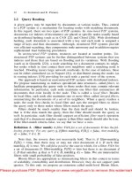
Figures 5(a) and 5(b) depict the error for the two algorithms as the amount of available
memory is increased. The Zipf parameters for the Zipfian distributions joined in Fig-
ures 5(a) and 5(b) are 1.0 and 1.5, respectively. The results for three settings of the shift
parameter are plotted in the graph of Figure 5(a), namely, 100, 200, and 300. On the
J
Please purchase PDF Split-Merge on www.verypdf.com to remove this watermark.
Processing Data-Stream Join Aggregates Using Skimmed Sketches
585
Fig. 5.
Results for Synthetic Data Sets: (a) (b)
other hand, smaller shifts of 30 and 50 are considered for the higher Zipf value of 1.5
in 5(b). This is because the data is more skewed when and thus, larger shift
parameter values cause the join size to become too small.
It is interesting to observe that the error of our skimmed-sketch algorithm is almost
an order of magnitude lower than the basic sketching technique for and several
orders of magnitude better when This is because as the data becomes more
skewed, the self-join sizes become large and this hurts the accuracy of the basic sketching
method. Our skimmed-sketch algorithm, on the other hand, avoids this problem by
eliminating from the sketches, the high frequency values. As a result, the self-join sizes
of the skimmed sketches never get too big, and thus the errors for our algorithm are
small (e.g., less than 10% for and almost zero when Also
, note that
the error typically increases with the shift parameter value since the join size is smaller
for larger shifts. Finally, observe that there is much more variance in the error for the

basic sketching method compared to our skimmed-sketch technique – we attribute this
to the high self-join sizes with basic sketching (recall that variance is proportional to the
product of the self-join sizes).
6
Conclusions
In this paper, we have presented the skimmed-sketch algorithm for estimating the join size
of two streams. (Our techniques also naturally extend to complex, multi-join aggregates.)
Our skimmed-sketch technique is the first comprehensive join-size estimation algorithm
to provide tight error guarantees while (1) achieving the lower bound on the space
required by any join-size estimation method, (2) handling general streaming updates, (3)
incurring a guaranteed small (i.e., logarithmic) processing overhead per stream element,
and (4) not assuming any a-priori knowledge of the data distribution. Our experimental
study with real-life as well as synthetic data streams has verified the superiority of our
skimmed-sketch algorithm compared to other known sketch-based methods for join-size
estimation.
Please purchase PDF Split-Merge on www.verypdf.com to remove this watermark.
586
S. Ganguly, M. Garofalakis, and R. Rastogi
References
1.
2.
3.
4.
5.
6.
7.
8.
9.
Greenwald, M., Khanna, S.: “Space-efficient online computation of quantile summaries”. In:
Proceedings of the 2001 ACM SIGMOD International Conference on Management of Data,

Santa Barbara, California (2001)
Gilbert, A., Kotidis, Y., Muthukrishnan, S., Strauss, M.: “How to Summarize the Universe:
Dynamic Maintenance of Quantiles”. In: Proceedings of the 28th International Conference
on Very Large Data Bases, Hong Kong (2002)
Alon, N., Matias, Y., Szegedy, M.: “The Space Complexity of Approximating the Frequency
Moments”. In: Proceedings of the 28th Annual ACM Symposium on the Theory of Computing,
Philadelphia, Pennsylvania (1996) 20–29
Alon, N., Gibbons, P.B., Matias, Y., Szegedy, M.: “Tracking Join and Self-Join Sizes in Limited
Storage”. In: Proceedings of the Eighteenth ACM SIGACT-SIGMOD-SIGART Symposium
on Principles of Database Systems, Philadeplphia, Pennsylvania (1999)
Dobra, A., Garofalakis, M., Gehrke, J., Rastogi, R.: “Processing Complex Aggregate Queries
over Data Streams”. In: Proceedings of the 2002 ACM SIGMOD International Conference
on Management of Data, Madison, Wisconsin (2002)
Gibbons, P.: “Distinct Sampling for Highly-accurate Answers to Distinct Values Queries and
Event Reports”. In: Proceedings of the 27th International Conference on Very Large Data
Bases, Roma, Italy (2001)
Cormode, G., Datar, M., Indyk, P., Muthukrishnan, S.: “Comparing Data Streams Using
Hamming Norms”. In: Proceedings of the 28th International Conference on Very Large Data
Bases, Hong Kong (2002)
Charikar, M., Chen, K., Farach-Colton, M.: “Finding frequent items in data streams”. In:
Proceedings of the 29th International Colloquium on Automata Languages and Programming.
(2002)
Cormode, G., Muthukrishnan, S.: “What’s Hot and What’s Not: Tracking Most Frequent Items
Dynamically”. In: Proceedings of the Twentysecond ACM SIGACT-SIGMOD-SIGART
Symposium on Principles of Database Systems, San Diego, California (2003)
Manku, G., Motwani, R.: “Approximate Frequency Counts over Data Streams”. In: Proceed-
ings of the 28th International Conference on Very Large Data Bases, Hong Kong (2002)
Gilbert, A.C., Kotidis, Y., Muthukrishnan, S., Strauss, M.J.: “Surfing Wavelets on Streams:
One-pass Summaries for Approximate Aggregate Queries”. In: Proceedings of the 27th
International Conference on Very Large Data Bases, Roma, Italy (2001)

Datar, M., Gionis, A., Indyk, P., Motwani, R.: “Maintaining Stream Statistics over Slid-
ing Windows”. In: Proceedings of the 13th Annual ACM-SIAM Symposium on Discrete
Algorithms, San Francisco, California (2002)
Vitter, J.: Random sampling with a reservoir. ACM Transactions on Mathematical Software
11 (1985) 37–57
Acharya, S., Gibbons, P.B., Poosala, V., Ramaswamy, S.: “Join Synopses for Approximate
Query Answering”. In: Proceedings of the 1999 ACM SIGMOD International Conference
on Management of Data, Philadelphia, Pennsylvania (1999) 275–286
Chakrabarti, K., Garofalakis, M., Rastogi, R., Shim, K.: “Approximate Query Processing
Using Wavelets”. In: Proceedings of the 26th International Conference on Very Large Data
Bases, Cairo, Egypt (2000) 111–122
Ganguly, S., Gibbons, P., Matias, Y., Silberschatz, A.: “Bifocal Sampling for Skew-Resistant
Join Size Estimation”. In: Proceedings of the 1996 ACM SIGMOD International Conference
on Management of Data, Montreal, Quebec (1996)
Ganguly, S., Garofalakis, M., Rastogi, R.: “Processing Data-Stream Join Aggregates Using
Skimmed Sketches”. Bell Labs Tech. Memorandum (2004)
10.
11.
12.
13.
14.
15.
16.
17.
Please purchase PDF Split-Merge on www.verypdf.com to remove this watermark.
Joining Punctuated Streams
Luping Ding, Nishant Mehta, Elke A. Rundensteiner, and George T. Heineman
Department of Computer Science, Worcester Polytechnic Institute
100 Institute Road, Worcester, MA 01609
{lisading , nishantm , rundenst , heineman}@cs.wpi.edu

Abstract. We focus on stream join optimization by exploiting the con-
straints that are dynamically embedded into data streams to signal the
end of transmitting certain attribute values. These constraints are called
punctuations. Our stream join operator,
PJoin,
is able to remove no-
longer-useful data from the state in a timely manner based on punc-
tuations, thus reducing memory overhead and improving the efficiency
o
f
probing. We equip PJoin with several alternate strategies for purging
the state and for propagating punctuations to benefit down-stream op-
erators. We also present an extensive experimental study to explore the
performance gains achieved by purging state as well as the trade-off be-
tween different purge strategies. Our experimental results of comparing
the performance of
PJoin
with XJoin, a stream join operator without a
constraint-exploiting mechanism, show that
PJoin
significantly outper-
forms XJoin with regard to both memory overhead and throughput.
1
Introduction
1.1
Stream Join Operators and Constraints
As stream-processing applications, including sensor network monitoring [14], on-
line transaction management [18], and online spreadsheets [9], to name a few,
have gained in popularity, continuous query processing is emerging as an impor-
tant research area [1] [5] [6] [15] [16]. The join operator, being one of the most

expensive and commonly used operators in continuous queries, has received in-
creasing attention [9] [13] [19]. Join processing in the stream context faces nu-
merous new challenges beyond those encountered in the traditional context. One
important new problem is the potentially unbounded runtime join state. Since
the join needs to maintain in its join state the data that has already arrived
in order to compare it against the data to be arriving in the future. As data
continuously streams in, the basic stream join solutions, such as symmetric hash
join [22], will indefinitely accumulate input data in the join state, thus easily
causing memory overflow.
XJoin [19] [20] extends the symmetric hash join to avoid memory overflow.
It moves part of the join state to the secondary storage (disk) upon running out
of memory. However, as more data streams in, a large portion of the join state
will be paged to disk. This will result in a huge amount of I/O operations. Then
the performance of XJoin may degrade in such circumstances.
E. Bertino et al. (Eds.): EDBT 2004, LNCS 2992, pp. 587–604, 2004.
© Springer-Verlag Berlin Heidelberg 2004
Please purchase PDF Split-Merge on www.verypdf.com to remove this watermark.
588
L. Ding et al.
In many cases, it is not practical to compare every tuple in a potentially
infinite stream with all tuples in another also possibly infinite stream [2]. In
response, the recent work on window joins [4] [8] [13] extends the traditional
join semantics to only join tuples within the current time windows. This way
the memory usage of the join state can be bounded by timely removing tuples
that drop out of the window. However, choosing an appropriate window size is
non-trivial. The join state may be rather bulky for large windows.
[3] proposes a k-constraint-exploiting join algorithm that utilizes statically
specified constraints, including clustered and ordered arrival of join values, to
purge the data that have finished joining with the matching cluster from the
opposite stream, thereby shrinking the state.

However, the static constraints only characterize restrictive cases of real-
world data. In view of this limitation, a new class of constraints called punc-
tuations [18] has been proposed to dynamically provide meta knowledge about
data streams. Punctuations are embedded into data streams (hence called punc-
tuated streams
)
to signal the end of transmitting certain attribute values. This
should enable stateful operators like join to discard partial join state during the
execution and blocking operators like group-by to emit partial results.
In some cases punctuations can be provided actively by the applications that
generate the data streams. For example, in an online auction management system
[18], the sellers portal merges items for sale submitted by sellers into a stream
called Open. The buyers portal merges the bids posted by bidders into another
stream called Bid. Since each item is open for bid only within a specific time
period, when the open auction period for an item expires, the auction system
can insert a punctuation into the Bid stream to signal the end of the bids for
that specific item.
The query system itself can also derive punctuations based on the semantics
of the application or certain static constraints, including the join between key
and foreign key, clustered or ordered arrival of certain attribute values, etc.
For example, since each tuple in the Open stream has a unique item_id value,
the query system can then insert a punctuation after each tuple in this stream
signaling no more tuple containing this specific item_id value will occur in the
future. Therefore punctuations cover a wider realm of constraints that may help
continuous query optimization. [18] also defines the rules for algebra operators,
including join, to purge runtime state and to propagate punctuations down-
stream. However, no concrete punctuation-exploiting join algorithms have been
proposed to date. This is the topic we thus focus on in this paper.
1.2
Our Approach: PJoin

In this paper, we present the first punctuation-exploiting stream join solution,
called PJoin. PJoin is a binary hash-based equi-join operator. It is able to ex-
ploit punctuations to achieve the optimization goals of reducing memory over-
head and of increasing the data output rate. Unlike prior stream join opera-
tors stated above,
PJoin
can also propagate appropriate punctuations to benefit
down-stream operators. Our contributions of
PJoin
include:
Please purchase PDF Split-Merge on www.verypdf.com to remove this watermark.
Joining Punctuated Streams
589
1.
2.
3.
4.
We propose alternate strategies for purging the join state, including eager
and lazy purge, and we explore the trade-off between different purge strate-
gies regarding the memory overhead and the data output rate experimentally.
We propose various strategies for propagating punctuations, including eager
and lazy index building as well as propagation in push and pull mode. We
also explore the trade-off between different strategies with regard to the
punctuation output rate.
We design an event-driven framework for accommodating all
PJoin compo-
nents, including memory and disk join, state purge, punctuation propaga-
tion, etc., to enable the flexible configuration of different join solutions.
We conduct an experimental study to validate our preformance analysis by
comparing the performance of PJoin with XJoin [19], a stream join operator

without a constraint-exploiting mechanism, as well as the performance of us-
ing different state purge strategies in terms of various data and punctuation
arrival rates. The experimental results show that
PJoin
outperforms XJoin
with regard to both memory overhead and data output rate.
In Section 2, we give background knowledge and a running example of punc-
tuated streams. In Section 3 we describe the execution logic design of
PJoin,
including alternate strategies for state purge and punctuation propagation. An
extensive experimental study is shown in Section 4. In Section 5 we explain re-
lated work. We discuss future extensions of PJoin
in Section 6 and conclude our
work in Section 7.
2
Punctuated Streams
2.1
Motivating Example
We now explain how punctuations can help with continuous query optimization
using the online auction example [18] described in Section 1.1. Fragments of
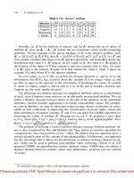
Open and Bid streams with punctuations are shown in Figure 1 (a). The query
in Figure 1 (b) joins all items for sale with their bids on item_id and then sum up
bid-increase values for each item that has at least one bid. In the corresponding
query plan shown in Figure 1 (c), an equi-join operator joins the Open stream
with the Bid stream on item_id. Our
PJoin operator can be used to perform this
equi-join. Thereafter, the group-by operator groups the output stream of the join
(denoted as by item_id. Whenever a punctuation from Bid is obtained
which signals the auction for a particular item is closed, the tuple in th
e state

for the Open stream that contains the same item_id value can then be purged.
Furthermore, a punctuation regarding this item_id value can be propagated to
the stream for the group-by to produce the result for this specific item.
2.2
Punctuations
Punctuation semantics. A punctuation can be viewed as a predicate on
stream elements that must evaluate to false for every element following the
Please purchase PDF Split-Merge on www.verypdf.com to remove this watermark.
590
L. Ding et al.
Fig. 1. Data Streams and Example Query.
punctuation, while the stream elements that appear before the punctuation can
evaluate either to true or to false. Hence a punctuation can be used to detect
and purge the data in the join state that won’t join with any future data.
In
PJoin, we use the same punctuation semantics as defined in [18], i.e., a
punctuation is an ordered set of patterns, with each pattern corresponding to an
attribute of a tuple. There are five kinds of patterns: wildcard, constant, range,
enumeration list and empty pattern. The “and” of any two punctuations is also
a punctuation. In this paper, we only focus on exploiting punctuations over the
join attribute. We assume that for any two punctuations and such that
arrives before if the patterns for the join attribute specified by and
are and respectively, then either or
We denote all tuples that arrived before time T from stream A and B
as tuple sets and respectively. All punctuations that arrived
before time T from stream A and B are denoted as punctuation sets
and respectively. According to [18], if a tuple has a join value that
matches the pattern declared by the punctuation then is said to match
denoted as If there exists a punctuation in such that
the tuple matches then is defined to also match the set denoted

as
Purge rules for join.
Given punctuation sets and
the purge
rules for tuple sets and are defined as follows:
Please purchase PDF Split-Merge on www.verypdf.com to remove this watermark.
Joining Punctuated Streams
591
Propagation rules for join. To propagate a punctuation, we must guarantee
that no more tuples that match this punctuation will be generated later. The
propagation rules are derived based on the following theorem.
if at time T, no tuple exists in such that then no tuple
such that
will be generated as a join result at or after time T
Proof by contradiction. Assume that at least one tuple such that
will be generated as a join result at or after time T. Then there must exist
at least one tuple in such that match Based on the
definition of punctuation, there will not be any tuple to be arriving from
stream A after time T such that Then must have been existing
in This contradicts the premise that no tuple exists in such
that Therefore, the assumption is wrong and no tuple such
that will be generated as a join result at or after time T. Thus
can be propagated safely at or after time T.
The propagation rules for and are then defined as follows:
3
PJoin Execution Logic
3.1
Components and Join State
Components. Join algorithms typically involve multiple subtasks, including:
(1) probe in-memory join state using a new tuple and produce result for any

match being found (memory join), (2) move part of the in-memory join state
to disk when running out of memory (state relocation), (3) retrieve data from
disk into memory for join processing (disk join), (4) purge no-longer-useful data
from the join state (state purge) and (5) propagate punctuations to the output
stream (punctuation propagation).
The frequencies of executing each of these subtasks may be rather different.
For example, memory join runs on a per-tuple basis, while state relocation exe-
cutes only when memory overflows and state purge is activated upon receiving
one or multiple punctuations. To achieve a fine-tuned, adaptive join execution,
we design separate components to accomplish each of the above subtasks. Fur-
thermore, for each component we explore a variety of alternate strategies that
can be plugged in to achieve optimization in different circumstances, as further
elaborated upon in Section 3.2 through Section 3.5. To increase the throughput,
several components may run concurrently in a multi-threaded mode. Section 3.6
introduces our event-based framework design for PJoin.
Theorem 1. Given and
for any punctuation
in
Please purchase PDF Split-Merge on www.verypdf.com to remove this watermark.
592
L. Ding et al.
Join
state.
Extending
from the
symmetric hash join [22],
PJoin
maintains
a
separate state for each input stream. All the above components operate on this

shared data storage. For each state, a hash table holds all tuples that have arrived
but have not yet been purged. Similar to XJoin [19], each hash bucket has an
in-memory portion and an on-disk portion. When memory usage of the join state
reaches a memory threshold, some data in the memory-resident portion will be
moved to the on-disk portion. A purge buffer contains the tuples which should
be purged based on the present punctuations, but cannot yet be purged safely
because they may possibly join with tuples stored on disk. The purge buffer will
be cleaned up by the disk join component. The punctuations that have arrived
but have not yet been propagated are stored in a punctuation set.
3.2
Memory Join and Disk Join
Due to the memory overflow resolution explained in Section 3.3 below, for each
new input tuple, the matching tuples in the opposite state could possibly reside in
two different places: memory and disk. Therefore, the join operation can happen
in two components. The memory join component will use the new tuple to probe
the memory-resident portion of the matching hash bucket of the opposite state
and produce the result, while the disk join component will fetch the disk-resident
portion of some or all the hash buckets and finish the left-over joins due to the
state relocation (Section 3.3). Since the disk join involves I/O operations which
are much more expensive than in-memory operations, the policies for scheduling
these two components are different. The memory join is executed on a per-tuple
basis. Only when the memory join cannot proceed due to the slow delivery of
the data or when punctuation propagation needs to finish up all the left-over
joins, will the disk join be scheduled to run. Similar to XJoin [19], we associate
an activation threshold with the disk join to model how aggressively it is to be
scheduled for execution.
3.3
State Relocation
PJoin employs the same memory overflow resolution as XJoin, i.e., moving part
of the state from memory to secondary storage (disk) when the memory becomes

full (reaches the memory threshold
)
. The corresponding component in
PJoin
is
called state relocation. Readers are referred to [19] for further details about the
state relocation.
3.4
State Purge
The state purge component removes data that will no longer contribute to any
future join result from the join state by applying the purge rules described in
Section 2. We propose two state purge strategies, eager (immediate) purge and
lazy (batch) purge. Eager purge starts to purge the state whenever a punctuation
is obtained. This can guarantee the minimum memory overhead caused by the
Please purchase PDF Split-Merge on www.verypdf.com to remove this watermark.
Joining Punctuated Streams
593
join state. Also by shrinking the state in an aggressive manner, the state probing
can be done more efficiently. However, since the state purge causes the extra
overhead for scanning the join state, when punctuations arrive very frequently
so that the cost of state scan exceeds the saving of probing, eager purge may
instead slow down the data output rate. In response, we propose a lazy purge
which will start purging when the number of new punctuations since the last
purge reaches a purge threshold, which is the number of punctuations to be
arriving between two state purges. We can view eager purge as a special case of
lazy purge, whose purge threshold is 1. Accordingly, finding an appropriate purge
threshold becomes an important task. In Section 4 we experimentally assess the
effect on PJoin performance posed by different purge thresholds.
3.5
Punctuation Propagation

Besides utilizing punctuations to shrink the runtime state, in some cases the
operator can also propagate punctuations to benefit other operators down-stream
in the query plan, for example, the group-by operator in Figure 1 (c). According
to the propagation rules described in Section 2, a join operator will propagate
punctuations
in a
lagged
fashion,
that
is,
before
a
punctuation
can be
released
to the output stream, the join must wait until all result tuples that match this
punctuation have been safely output. Hence we consider to initiate propagation
periodically. However, each time we invoke the propagation, each punctuation
in the punctuation sets needs to be evaluated against all tuples currently in the
same state. Therefore, the punctuations which were not able to be propagated
in the previous propagation run may be evaluated against those tuples that
have already been compared with last time, thus incurring duplicate expression
evaluations. To avoid this problem and to propagate punctuations correctly, we
design an incrementally maintained punctuation index which arranges the data
in the join state by punctuations.
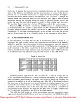
Punctuation index. To construct a punctuation index (Figure 2 (c)), each
punctuation in the punctuation set is associated with a unique ID (pid) and a
count recording the number of matching tuples that reside in the same state
(Figure 2 (a)). We also augment the structure of each tuple to add the pid
which denotes the punctuation that matches the tuple (Figure 2 (b)). If a tuple

matches multiple punctuations, the pid of the tuple is always set as the pid of
the first arrived punctuation found to be matched. If the tuple is not valid for
any existing punctuations, the pid of this tuple is null. Upon arrival of a new
punctuation only tuples with pid field being null need to be evaluated against
Therefore the punctuation index is constructed incrementally so to avoid the
duplicate expression evaluations. Whenever a tuple is purged from the state, the
punctuation whose pid corresponds the pid contained by the purged tuple will
deduct its count field. When the count of a punctuation reaches 0 which means
no tuple matching this punctuation exists in the state, according to Theorem
1 in Section 2, this punctuation becomes propagable. The punctuations being
propagated are immediately removed from the punctuation set.
Please purchase PDF Split-Merge on www.verypdf.com to remove this watermark.
594
L. Ding et al.
Fig. 2. Data Structures for Punctuation Propagation.
Algorithms for index building and propagation. We can see that punctua-
tion propagation involves two important steps: punctuation index building which
associates each tuple in the join state with a punctuation and propagation which
outputs the punctuations with the count field being zero. Clearly, propagation
relies on the index building process. Figure 3 shows the algorithm for construct-
ing a punctuation index for tuples from stream B (Lines 1-14) and the algorithm
for propagating punctuations from stream B to the output stream (Lines 16-21).
Fig. 3.
Algorithms of Punctuation Index Building and Propagation.
Eager and lazy index building. Although our incrementally constructed
punctuation index avoids duplicate expression evaluations, it still needs to scan
the entire join state to search for the tuples whose pids are null each time it
is executed. We thus propose to batch the index building for multiple punctu-
ations in order to share the cost of scanning the state. Accordingly, instead of
Please purchase PDF Split-Merge on www.verypdf.com to remove this watermark.

Joining Punctuated Streams
595
triggering the index building upon the arrival of each punctuation, which we
call eager index building, we run it only when the punctuation propagation is
invoked, called lazy index building. However, eager index building is still pre-
ferred in some cases. For example, it can help guarantee the steady instead of
bursty output of punctuations whenever possible. In the eager approach, since
the index is incrementally built right upon receiving each punctuation and the
index is indirectly maintained by the state purge, some punctuations may be
detected to be propagable much earlier than the next invocation of propagation.
Propagation mode.
PJoin is able to trigger punctuation propagation in either
push or pull mode. In the push mode, PJoin actively propagates punctuations
when either a fixed time interval since the last propagation has gone by, or a
fixed number of punctuations have been received since the last propagation. We
call them time propagation threshold and count propagation threshold respec-
tively. On the other hand, PJoin is also able to propagate punctuations upon the
request of the down-stream operators, which would be the beneficiaries of the
propagation. This is called the pull mode.
3.6
Event-Driven Framework of PJoin
To implement the PJoin execution logic described above, with components being
tunable, a join framework which incorporates the following features is desired.
1.
2.
The framework should keep track of a variety of runtime parameters that
serve as the triggering conditions for executing each component, such as the
size of the join state, the number of punctuations that arrived since the
last state purge, etc. When a certain parameter reaches the corresponding
threshold, such as the purge threshold, the appropriate components should

be scheduled to run.
The framework should be able to model the different coupling alternatives
among components and easily switch from one option to another. For ex-
ample, the lazy index building is coupled with the punctuation propagation,
while the eager index building is independent of the punctuation propagation
strategy selected by a given join execution configuration.
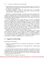
To accomplish the above features, we have designed an event-driven frame-
work for
PJoin as shown in Figure 4. The memory join runs as the main thread.
It continuously retrieves data from the input streams and generates results. A
monitor is responsible for keeping track of the status of various runtime pa-
rameters about the input streams and the join state being changed during the
execution of the memory join. Once a certain threshold is reached, for example
the size of the join state reaches the memory threshold or both input streams are
temporarily stuck due to network delay and the disk join activation threshold
is reached, the monitor will invoke the corresponding event. Then the listeners
of the event, which may be either disk join, state purge, state relocation, in-
dex build or punctuation propagation component, will start running as a second
thread. If an event has multiple listeners, these listeners will be executed in an
order specified in the event-listener registry described below.
Please purchase PDF Split-Merge on www.verypdf.com to remove this watermark.
596
L. Ding et al.
Fig. 4. Event-Driven Framework of PJoin.
The following events have been defined to model the status changes of mon-
itored runtime parameters that may cause a component to be activated.
1.
2.
3.
4.

5.
6.
7.
StreamEmptyEvent signals both input streams run out of tuples.
PurgeThresholdReachEvent signals the purge threshold is reached.
StateFullEvent signals the size of the in-memory join state reaches the mem-
ory threshold.
NewPunctReadyEvent signals a new punctuation arrives.
PropagateRequestEvent signals a propagation request is received from down-
stream operators.
Propagate
TimeExpireEvent signals the time propagation threshold is reached.
PropagateCountReachEvent signals the count propagation threshold is
reached.
PJoin
maintains an event-listener registry. Each entry in the registry lists the
event to be generated, the additional conditions to be checked and the listeners
(components) which will be executed to handle the event. The registry while
initiated at the static query optimization phase can be updated at runtime. All
parameters for invoking the events, including the purge, memory and propagation
threshold, are specified inside the monitor and can also be changed at runtime.
Table 1 gives an example of this registry. This configuration of
PJoin
is used
by several experiments shown in Section 4. In this configuration, we apply the
lazy purge strategy, that is, to purge state whenever the purge threshold is
reached. Also the lazy index building and the push mode propagation are ap-
plied, that is, when the count propagation threshold is reached, we first con-
struct the punctuation index for all newly-arrived punctuations since the last
index building and then start propagation.

Please purchase PDF Split-Merge on www.verypdf.com to remove this watermark.
Joining Punctuated Streams
597
Fig. 5. PJoin vs. XJoin, Memory Over-
head, Punctuation Inter-arrival: 40 tu-
ples/punctuation.
Fig. 6. PJoin Memory Overhead, Punc-
tuation Inter-arrival: 10, 20, 30 tu-
ples/punctuation.
4
Experimental Study
We have implemented the PJoin operator in Java as a query operator in the
Raindrop XQuery subscription system [17] based on the event-based framework
presented in Section 3.6. Below we describe the experimental study we have
conducted to explore the effectiveness of our punctuation-exploiting stream join
optimization. The test machine has a 2.4GHz Intel(R) Pentium-IV processor
and a 512MB RAM, running Windows XP and Java 1.4.1.01 SDK. We have
created a benchmark system to generate synthetic data streams by controlling
the arrival patterns and rates of the data and punctuations. In all experiments
shown in this section, the tuples from both input streams have a Poisson inter-
arrival time with a mean of 2 milliseconds. All experiments run a many-to-many
join over two input streams, which, we believe, exhibits the most general cases
of our solution. In the charts, we denote the PJoin with purge threshold as
Accordingly, PJoin using eager purge is denoted as PJoin-1.
4.1
PJoin versus XJoin
First we compare the performance of PJoin with XJoin [19], a stream join oper-
ator without a constraint-exploiting mechanism. We are interested in exploring
two questions: (1) how much memory overhead can be saved and (2) to what
degree can the tuple output rate be improved. In order to be able to compare

these two join solutions, we have also implemented XJoin in our system and
applied the same optimizations as we did for PJoin.
To answer the first question, we compare PJoin using the eager purge with
XJoin regarding the total number of tuples in the join state during the length of
the execution. The input punctuations have a Poisson inter-arrival with a mean
of 40 tuples/punctuation. From Figure 5 we can see that the memory requirement
for the
PJoin
state is almost insignificant compared to that of XJoin.
As the punctuation inter-arrival increases, the size of the PJoin state will
increase accordingly. When the punctuation inter-arrival reaches infinity so that
Please purchase PDF Split-Merge on www.verypdf.com to remove this watermark.
598
L. Ding et al.
Fig. 7.
PJoin vs. XJoin, Tuple Output Rates, Punctuation Inter-arrival: 30 tu-
ples/punctuation.
no punctuations exist in the input stream, the memory requirement of PJoin
becomes the same as that of XJoin.
In Figure 6, we vary the punctuation inter-arrival to be 10, 20 and 30 tu-
ples/punctuation respectively for three different runs of PJoin accordingly. We
can see that as the punctuation inter-arrival increases, the average size of the
PJoin state becomes larger correspondingly.
To answer the second question, Figure 7 compares the tuple output rate of
PJoin to that of XJoin. We can see that as time advances, PJoin maintains an
almost steady output rate whereas the output rate of XJoin drops. This decrease
in XJoin output rate occurs because the XJoin state increases over time thereby
leading to an increasing cost for probing state. From this experiment we conclude
that PJoin performs better or at least equivalent to XJoin regarding both the
output rate and the memory resources consumption.

4.2
State Purge Strategies for PJoin
No
w
we explore how the performance of PJoin is affected by different state purge
strategies. In this experiment, the input punctuations have a Poisson inter-arrival
with a mean of 10 tuples/punctuation. We vary the purge threshold to start
purging state after receiving every 10, 100, 400, 800 punctuations respectively
and measure its effect on the output rate and memory overhead of the join.
Figure 8 shows the state requirements for the eager purge (PJoin-1) and the
lazy purge with purge threshold 10 (PJoin-10). The chart confirms that the eager
purge is the best strategy for minimizing the join state, whereas the lazy purge
requires more memory to operate.
Figure 9 compares the PJoin output rate using different purge strategies. We
plot the number of output tuples against time summarized over four experiment
runs, each run with a different purge threshold (1,100,400 and 800 respectively).
We can see that up to some limit, the higher the purge threshold, the higher
the output rate. This is because there is a cost associated with purge, and thus
purging very frequently such as the eager strategy leads to a loss in performance.
But this gain in output rate is at the cost of the increase in memory overhead.
Please purchase PDF Split-Merge on www.verypdf.com to remove this watermark.
Joining Punctuated Streams
599
Fig. 8. Eager vs. Lazy Purge, Memory
Overhead, Punctuation Inter-arrival: 10
tuples/punctuation.
Fig. 9. Eager vs. Lazy Purge, Tuple Out-
put rates, Punctuation Inter-arrival: 10 tu-
ples/punctuation
.

Fig. 10. Memory Overhead, Asymmet-
ric Punctuation Inter-arrival Rates,
A Punctuation Inter-arrival: 10 tu-
ples/punctuation, B Punctuation Inter-
arrival: 20, 30, 40 tuples/punctuation.
Fig. 11. Tuple Output Rates, Asym-
metric Punctuation Inter-arrival Rates,
A Punctuation Inter-arrival: 10 tu-
ples/punctuation, B Punctuation Inter-
arrival: 20, 40 tuples/punctuation.
When the increased cost of probing the state exceeds the cost of purge, we start
to lose on performance, such as the case of PJoin-400 and PJoin-800. This is the
same problem as encountered by XJoin, that is, every new tuple enlarges the
state, which in turn increases the cost of probing the state.
4.3
Asymmetric Punctuation Inter-arrival Rate
Now we explore the performance of
PJoin
in terms of input streams with
asymmetric punctuation inter-arrivals. We keep the punctuation inter-arrival of
stream A constant at 10 tuples/punctuation and vary that of stream B. Figure
10 shows the state requirement of PJoin using eager purge. We can see that the
larger the difference in the punctuation inter-arrival of the two input streams, the
larger will be the memory requirement. Less frequent punctuations from stream
B cause the A state to be purged less frequently. Hence the A state becomes
larger.
Please purchase PDF Split-Merge on www.verypdf.com to remove this watermark.
600
L. Ding et al.
Fig. 12. Eager vs. Lazy Purge, Out-

put Rates, Asymmetric Punctuation Inter-
arrival Rates, A Punctuation Inter-arrival:
10 tuples/punctuation, B Punctuation
Inter-arrival: 20 tuples/punctuation.
Fig. 13. Eager vs. Lazy Purge, Mem-
ory Overhead, Asymmetric Punctuation
Inter-arrival Rates, A Punctuation Inter-
arrival: 10 tuples/punctuation, B Punctu-
ation Inter-arrival: 20 tuples/punctuation.
Another interesting phenomenon not shown here is that the B state is very
small or insignificant compared to the A state. This happens because punctu-
ations from stream A arrive at a faster rate. Thus most of the time when a B
tuple is received, there already exists an A punctuation that can drop this B
tuple on the fly [7]. Therefore most B tuples never become a part of the state.
Figure 11 gives an idea about the tuple output rate of PJoin for the above
cases. The slower the punctuation arrival rate, the greater is the tuple output
rate. This is because the slow punctuation arrival rate means a smaller number
of purges and hence the less overhead caused by purge.
Figure 12 shows the comparison of
PJoin against XJoin in terms of asymmet-
ric punctuation inter-arrivals. The punctuation inter-arrival of stream A is 10
tuples/punctuation and that of stream B is 20 tuples/punctuation. We can see
that the output rate of
PJoin with the eager purge (PJoin-1) lags behind that of
XJoin. This is mainly because of the cost of purge associated with PJoin. One
way to overcome this problem is to use the lazy purge together with an appropri-
ate setting of the purge threshold. This will make the output rate of
PJoin better
or at least equivalent to that of XJoin. Figure 13 shows the state requirements
for this case. We conclude that if the goal is to minimize the memory overhead

of the join state, we can use the eager purge strategy. Otherwise the lazy purge
with an appropriate purge threshold value can give us a significant advantage in
tuple output rate, at the expense of insignificant increase in memory overhead.
4.4
Punctuation Propagation
Lastly, we test the punctuation propagation ability of PJoin. In this experi-
ment, both input streams have a punctuation inter-arrival with a mean of 40
tuples/punctuation. We show the ideal case in which punctuations from both
input streams arrive in the same order and of same granularity, i.e., each punc-
tuation contains a constant pattern. PJoin is configured to start propagation after
a pair of equivalent punctuations has been received from both input streams.
Please purchase PDF Split-Merge on www.verypdf.com to remove this watermark.
Joining Punctuated Streams
601
Fig. 14.
Punctuation Propagation, Punctuation Inter-arrival: 40 tuples/punctuation
Figure 14 shows the number of punctuations being output over time. We can
see that PJoin can guarantee a steady punctuation propagation rate in the ideal
case. This property can be very useful for the down-stream operators such as
group-by that themselves rely on the availability of input punctuations.
5
Related Work
As the data being queried has expanded from finite and statically available
datasets to distributed continuous data streams ([1] [5] [6] [15]), new problems
have arisen. Specific to the join processing, two important problems need to
be tackled: potentially unbounded growing join state and dynamic runtime fea-
tures of data streams such as widely-varying data arrival rates. In response, the
constraint-based join optimization [16] and intra-operator adaptivity [11] [12] are
proposed in the literature to address these two issues respectively.
The main goal of constraint-based join optimization is to in a timely manner

detect and purge the no-longer-useful data from the state. Window joins exploit
time-based constraints called sliding windows to remove the expired data from
the state whenever a time window passes. [1] defines formal semantics for a bi-
nary join that incorporates a window specification. Kang et al. [13] provide a
unit-time-basis cost model for analyzing the performance of a binary window
join. They also propose strategies for maximizing the join efficiency in various
scenarios. [8] studies algorithms for handling sliding window multi-join process-
ing. [10] researches the shared execution of multiple window join operators. They
provide alternate strategies that favor different window sizes. The
algorithm [3] exploits clustered data arrival, a value-based constraint
to help detect stale data. However, both window and k-constraints are statically
specified, which only reflect the restrictive cases of the real-world data.
Punctuations [18] are a new class of constraints embedded into the stream dy-
namically at runtime. The static constraints such as one-to-many join cardinality
and clustered arrival of join values can also be represented by punctuations. Be-
yond the general concepts of punctuations, [18] also lists all rules for algebra
Please purchase PDF Split-Merge on www.verypdf.com to remove this watermark.