Tài liệu Handbook of Neural Network Signal Processing P2 docx
Bạn đang xem bản rút gọn của tài liệu. Xem và tải ngay bản đầy đủ của tài liệu tại đây (950.34 KB, 20 trang )
Assume that g
i
(x) = 1 (hence g
k
(x) = 0,k = i), update the expert i based on output error.
Update gating network so that g
i
(x) is even closer to unity.
Alternatively, a batch training method can be adopted:
1. Apply a clustering algorithm to cluster the set of training samples into n clusters. Use
the membership information to train the gating network.
2. Assign each cluster to an expert module and train the corresponding expert module.
3. Fine-tune the performance using gradient-based learning.
Note that the function of the gating network is to partition the feature space into largely disjointed
regions and assign each region to an expert module. In this way, an individual expert module only
needs to learn a subregion in the feature space and is likely to yield better performance.
Combining n expert modules under the gating network, the overall performance is expected to
improve. Figure 1.19 shows an example using the batch training method presented above. The
dots are the training and testing samples. The circles are the cluster centers that represent individual
experts. These cluster centers are found by applying the k-means clustering algorithm on the training
samples. The gating network output is proportional to the inverse of the square distance from each
sample to all three cluster centers. The output value is normalized so that the sum equals unity.
Each expert module implements a simple linear model (a straight line in this example). We did
not implement the third step, so the results are obtained without fine-tuning. The corresponding
MATLAB m-files are moedemo.m and moegate.m.
1.19 Illustration of mixture of expert network using batched training method.
1.2.6 Support Vector Machines (SVMs)
A support vector machine [14] has a basic format, as depicted in Figure 1.20, whereϕ
k
(x) is a
nonlinear transformation of the input feature vector x into a high-dimensional space new feature
vector ϕ(x) =[ϕ
1
(x)ϕ
2
(x)...ϕ
p
(x)]. The output y is computed as:
y(x) =
p
k=1
w
k
ϕ
k
(x) + b = ϕ(x)w
T
+ b
where w =[w
1
w
2
...w
p
] is the 1 × p weight vector, and b is the bias term. The dimension of
ϕ(x)(= p) is usually much larger than that of the original feature vector (= m). It has been argued
© 2002 by CRC Press LLC
that mapping a low-dimensional feature into a higher-dimensional feature space will likely make the
resulting feature vectors linearly separable. In other words, using ϕ as a feature vector is likely to
result in better pattern classification results.
1.20 An SVM neural network structure.
Given a set of training vectors {x(i); 1 ≤ i ≤ N}, one can solve the weight vector w as:
w =
N
i=1
γ
i
ϕ(x(i)) = γ
where =[ϕ(x(1)) ϕ(x(2)) ...ϕ(x(N ))]
T
is an N ×p matrix, and γ isa1×N vector. Substituting
w into y(x) yields:
y(x) = ϕ(x)w
T
+ b =
N
i=1
γ
i
ϕ(x)ϕ
T
(x(i)) + b =
N
i=1
γ
i
K(x, x(i)) + b
where the kernel K(x, x(i)) is a scalar-valued function of the testing sample x and a training sample
x(i).ForN<<p, one may choose to use γ and K(x, x(i)) to evaluate y(x) instead of using w and
ϕ(x) explicitly. For this purpose, one must estimate γ and b and identify a set of support vectors
{x(i); 1 ≤i≤N} that may be a subset of the entire training set of data samples.
Commonly used kernel functions are summarized in Table 1.4.
TABLE 1.4 List of Commonly Used Kernel Functions for Support Vector Machines (SVMs)
Type of SVM
K(x, y)
Comments
Polynomial learning machine
x
T
y + 1
p
p
: selected a priori
Radial basis function
exp
−
1
2σ
2
x − y
2
σ
2
: selected a priori
Two-layer perceptron
tanh
β
o
x
T
y + β
1
Only some
β
o
and
β
1
values are feasible
© 2002 by CRC Press LLC
1.21 A linearly separable pattern classification example.
ρ
is the distance between each class to the decision boundary.
To identify the support vectors from a set of training data samples, consider the linearly separable
pattern classification example shown in Figure 1.21. According to Cortes and Vapnik [15], the
empirical risk is minimized in a linearly separable two-class pattern classification problem, as shown
in Figure 1.21, if the decision boundary is located such that the minimum distance from each training
sample of each class to the decision boundary is maximized. In other words, the parameter ρ in
Figure 1.21 should be maximized subject to the constraints that all “o” class samples should be on
one side of the decision boundary, and all “x” class samples should be on the other side of the decision
boundary. This can be formulated as a nonlinear constrained quadratic optimization problem. Using
a Karush–Kühn–Tucker condition, it can be shown that not all training samples will contribute to
the determination of the decision boundary. In fact, as shown in Figure 1.21, only those training
samples that are closest to the decision boundary (marked with color in the figure) will contribute to
the solution of w and b. These training samples will then be identified as the support vectors.
There are many public domain implementations of SVM. They include a support vector machine
MATLAB toolbox (
), aCimplementationSVM_light( />thorsten/svm_light/), andarecentreleaseofBSVM( Figure1.22
shows an example using an SVM toolbox to solve a linearly separable problem with a radial basis
kernel. The three support vectors are labeled with white dots and the decision boundary and the gap
are also illustrated.
1.3 Neural Network Solutions to Signal Processing Problems
1.3.1 Digital Signal Processing
In the most general sense a signal is a physical quantity that is a function of one or more independent
variables such as time or spatial coordinates. A signal can be naturally occurring or artificially
synthesized. It can be the temperature variations in a building, a stock price quote, the faint radiation
from a distant galaxy, or the brain waves from a human body.
How do we use the signals obtained from various measurements? Simply put, a signal carries
information. Based on building temperature readings, we may turn the building’s heater on or off.
Based on a stock price quote, we may buy or sell stocks. The faint radiation from a distant galaxy may
reveal the secret of the universe. Brain waves from a human body may be used to communicate and
control external devices. In short, the purpose of signal processing is to exploit inherent information
© 2002 by CRC Press LLC
1.22 Illustration of support vector machine classification result.
carried by the signal. More specifically, by processing a signal, we can manipulate the information by
injecting new information into the signal or by extracting inherent information from the signal. There
are many ways to process signals. One may filter, transform, transmit, estimate, detect, recognize,
synthesize, record, or reproduce a signal.
Perhaps the most comprehensive definition of signal processing is the Field of Interests statement
of the IEEE (Institute of Electrical and Electronics Engineering) Signal Processing Society, which
states that signal processing concerns
... theory and application of filtering, coding, transmitting, estimating, detecting,
analyzing, recognizing, synthesizing, recording, and reproducing signals by digital or
analog devices or techniques. The term “signal” includes audio, video, speech, image,
communications, geophysical, sonar, radar, medical, musical, and other signals.
If a signal is a function of time only, it is a one-dimensional signal. If the time variable is continuous,
the corresponding signal is a continuous time signal. Most real world signals are continuous time
signals. A continuous time signal can be sampled at regular time intervals to yield a discrete time
signal. A discrete time signal can be described using a sequence of numbers. To process a discrete
time signal using digital computers, the value of each discrete time sample may also be quantized to
finite precision to fit into the internal word length of the computer.
1.3.1.1 A Taxonomy of Digital Signal Processing (DSP) Algorithms
A DSP algorithm describes how to process a given signal. Depending on their assumptions
of the underlying signal, the mathematical formulations, DSP algorithms can be characterized in a
number of different dimensions:
Deterministic vs. statistical signal processing — In a statistical DSP algorithm, it is assumed
that the underlying signal is generated from a probabilistic model. No such model is assumed in a
deterministic DSP algorithm. Almost all the neural network application examples we encountered
concerned statistical signal processing applications.
© 2002 by CRC Press LLC
Linear vs. nonlinear signal processing — A linear signal processing algorithm is a linear system
(linear operator) operating on the incoming signal. If a particular signal is a weighted sum of
two different signals, then the output of this signal after applying a linear operator will also be a
weighted sum of the outputs of those two different signals. This superimposition property is unique
to linear signal processing algorithms. Neural network applications to signal processing are mostly
for nonlinear signal processing algorithms.
Data-adaptive vs. data-independent formulation — A data-independent signal processing algo-
rithm has fixed parameters that do not depend on specific data samples to be processed. On the
other hand, a data-adaptive algorithm will adjust its parameters based on the signal presented to
the algorithm. Thus, data-adaptive algorithms need a training phase to acquire specific values of
parameters. Most neural network based signal processing algorithms are data adaptive.
Memoryless vs. dynamic system — The output of a signal processing algorithm may depend on both
the present input signal as well as a signal in the past. Usually, the signal in the past is summarized
as a state vector. Such a system is called a dynamic system that has memory (remembering the past).
A memoryless system’s output is dependent only on the present input. While linear dynamic system
theory has been well developed, nonlinear dynamic system theory that incorporates neural networks
is still an ongoing research area.
1.3.1.2 Nonlinear Filtering
There are many reports on using artificial neural networks to perform nonlinear filtering of a
signal for the purposes of noise reduction and signal enhancement. However, due to the nonlinear
nature, most applications must be developed for specific training corpus and are data dependent.
Therefore, to apply ANN for nonlinear filtering, one must be able to collect an extensive set of
training samples to cover all possible situations and develop a neural network to adapt to the given
training set.
For example [16], an MLP-based neural filter is developed to remove quantum noise from X-ray
images, while at the same time trying to enhance the edge of the images. The purpose is to replace
current high dosage X-ray film with low dosage X-ray while improving the quality of the image.
In this application, high dosage X-ray film with high-pass filtered edge enhancement is used as the
target. A simulated low-dosage X-ray image, derived from the original high-dosage X-ray image, is
used as the input to the MLP. The resulting SNR improvement of a testing data set is used to gauge
the effectiveness of this approach.
1.3.1.3 Linear Transformations
A linear transformation transforms a block (vector) of signal into a different vector space where
special properties may be exploited. For example, a discrete Fourier transform transforms a time
domain signal into frequencies in the frequency domain. A discrete wavelet transform transforms
to and back from scale space representation of the signal. A very important application of linear
transformation is the transform-based signal compression. The original signal is first transformed
using a linear transformation such as the fast Fourier transform, the discrete cosine transform, or the
discrete wavelet transform into the frequency domain. The purpose is to compact the energy in the
original signal into a few large frequency coefficients. By encoding these very few large frequency
coefficients, the original signal can be compressed with a high compression ratio.
Another popular data-dependent linear transform is called principal component analysis (PCA)
or, sometimes, Karhunen–Loeve expansion (KL expansion). The main difference between PCA and
other types of linear transforms is that the transformation depends on the inherent structure of the
data. Hence, PCA can achieve optimal performance in terms of energy compaction. The generalized
© 2002 by CRC Press LLC
Hebbian learning neural network structure can be regarded as an online approximation of PCA, and
hence can be applied to tasks that would require PCA.
1.3.1.4 Pattern Classification
Pattern classification is perhaps the most important application of artificial neural networks.
In fact, a majority of neural network applications can be categorized as solving complex pattern
classification problems. In the area of signal processing, pattern classification has been employed in
speech recognition, optical (handwritten) character recognition, bar code recognition, human face
recognition, fingerprint recognition, radar/sonar target identification, biomedical signal diagnosis,
and numerous other areas.
Given a set of feature vectors {x; x ∈
n
} of an object of interest, we assume that the (probabilistic)
state of nature of each object can be designated with a label ω ∈ , where is the set of all possible
labels. We denote the prior probability p(ω) to be the probability that a feature vector is assigned
by nature of the object to the label ω
c
. We may also define a posterior probability p(ω|x) to be the
probability that a feature vector x has label ω
c
given the observation of the feature vector x.
A minimum error statistical pattern classifier is one that maps each feature vector x to an element
in such that the probability that the mapped label is different from the label assigned by the nature
of the object (the probability of misclassification) is minimized. To achieve this minimum error rate,
for a given feature vector x, one must
Decide x has label ω
i
if p(ω
i
|x)>p(ω
j
|x) for j = i, ω
i
,ω
j
∈ .
In practice, it is very difficult to evaluate the posterior probability in close form. Instead, one may
use an appropriate discriminant function g
i
(x) that satisfies
g
i
(x)>g
j
(x) if p(ω
i
|x)>p(ω
j
|x) for j = i, ω
i
,ω
j
∈ .
Then, the minimum error pattern classification can be achieved by
Decide x has label ω
i
if g
i
(x)>g
j
(x) for j = i, ω
i
, ∈ .
The minimum probability of misclassification is also known as the Bayes error, and a minimum error
classifier is also known as a maximum a posteriori probability (MAP) classifier.
In applying the MAP classifier to real world applications, one must find an estimate of the posterior
probability p(ω|x) or, equivalently, a discriminant function g(x) based on a set of training data. Thus,
a neural network such as the multilayer perceptron can be a good candidate for such a purpose. A
support vector machine is another neural network structure that directly estimates a discriminant
function.
One may apply the Bayes rule to express the posterior probability as:
p(ω|x) = p(x|ω)p(ω)/p(x)
where p(x|ω) is called the likelihood function, p(ω) is the prior probability distribution of class label
ω, and p(x) is the marginal probability distribution of the feature vector x. Since p(x) is independent
of ω
i
, the MAP decision rule can be expressed as:
Decide x has label ω
i
if p(x|ω
i
)p(ω
i
)>p(x|ω
j
)p(ω
j
) for j = i, ω
i
,ω
j
∈ .
p(ω
i
) can be estimated from the training data samples as the percentage of training samples that are
labeled ω
i
. Thus, only the likelihood function needs to be estimated. One popular model for such a
purpose is a mixture of the Gaussian model:
p
(
x|ω
i
)
=
K
i
k=1
ν
ki
exp
−
(
x − m
ki
)
2
/
2σ
2
ki
.
© 2002 by CRC Press LLC
To deduce the model parameters, {(ν
ki
, m
ki
,σ
2
ki
); 1 ≤ k ≤ K
i
, 1 ≤ i ≤ C} (C =||). Obviously, a
radial basis neural network structure will be handy here to model the mixture of Gaussian likelihood
function.
Since the weighted sum of the mixture of Gaussian density functions is still a mixture of a Gaussian
density function, one may choose instead to model the marginal distribution p(x) with a mixture of
a Gaussian model. Each individual Gaussian density function in the mixture model will be assigned
to a particular class label based on a majority voting of training samples assigned to that particular
Gaussian density function. Additional fine-tuning can be applied to enhance the probability of
classification. This is the approach implemented in the learning vector quantization (LVQ) neural
network. The above discussion is summarized in Table 1.5.
TABLE 1.5 Pattern Classification Methods and Corresponding Neural
Network Implementations
Pattern Classification Methods Neural Network
Implementations
MAP: maximize posterior probability
p(ω|x)
Multilayer perceptron
MAP: maximize discriminant function
g(x)
Support vector machine
ML: maximize product of likelihood function and prior Radial basis network, LVQ
distribution
p(x|ω)p(ω)
1.3.1.5 Detection
Detection can be regarded as a special case of pattern classification where only two class labels
are used: detect or no-detect. The purpose of signal detection is to detect the presence of a known
signal in the presence of additive noise. It is assumed that the received signal (often a vector) x may
consist of the true signal vector s and an additive statistical noise vector n:
x = s + n
or simply the noise vector:
x = n .
Assuming that the probability density function of the noise vector n is known, one may apply
statistical hypothesis testing procedure to determine whether x contains the known signal s.For
example, we may calculate the log-likelihood function and compare it to a predefined threshold in
order to maximize the probability of detection subject to an upper bound of a prespecified false alarm
rate.
One popular assumption is that the noise vector n has a multivariate Gaussian distribution with
zero mean and known covariance matrix. In this case, the inner product s
T
x is a sufficient statistic,
known as a matched filter signal detector.
A single neuron perceptron can be used to implement the matched filter computation. The signal
template s will be the weight vector, and the observation x is applied as its input. The bias term is
threshold, and the output = 1 if the presence of the signal is detected. A multilayer perceptron can
also be used to implement a nonlinear matched filter if the output activation function is a threshold
function. By the same token, a support vector machine is also a plausible neural network structure
to realize a nonlinear matched filter.
1.3.1.6 Time Series Modeling
A time series is a sequence of readings as a function of time. It arises in numerous practical
applications, including stock prices, weather readings (e.g., temperature), utility demand, etc. A
© 2002 by CRC Press LLC
central issue in time series modeling is to predict the future time series outcomes. There are three
different ways of predicting a time series {y(t)}:
1. Predicting y(t) based on past observations {y(t − 1), y(t − 2),...}. That is,
ˆy(t) = E{y(t)|y(t − 1), y(t − 2),...} .
2. Predicting y(t) based on observation of other relevant time series {x(t); x(t), x(t − 1),...}:
ˆy(t) = E{y(t)|x(t), x(t − 1), x(t − 2),...} .
3. Predicting y(t + 1) based on both {y(t − k); k = 1, 2,...} and {x(t − m); m = 0, 1, 2,...}:
ˆy(t) = E{y(t)|x(t), x(t − 1), x(t − 2),...,y(t − 1), y(t − 2),...} .
Both {x(t)} and {y(t)} can be vector valued time series. If the conditional expectation is a linear
function, then these formulae lead to three popular linear time series models:
Auto-regressive (AR)
y(t) =
N
k=1
a(k)y(t − k) + e(t)
Moving average (MA)
y(t) =
M
m=0
b(m)x(t − m)
Auto-regressive moving average (ARMA)
y(t) =
M
m=0
b(m)x(t − m) +
N
k=1
a(k)y(t − k) + e(t)
In the AR and ARMA models, e(t) is a zero-mean, uncorrelated innovation process representing
a random persistent excitation of the system. Neural network models can be incorporated into
these time series models to facilitate nonlinear time series prediction. Specifically, one may use the
generalized state vector s as an input to a neural network and obtain the output y(t) from the output
of the neural network.
One such example is the time-delayed neural network (TDNN) that can be described as:
y(n) = ϕ(x(n), x(n − 1),...,x(n− M))
ϕ(•) is a nonlinear transformation of its arguments, and it is implemented with a multilayer perceptron
in TDNN.
1.3.1.7 System Identification
System identification is a modeling problem. Given a black box system, the goal of system
identification is to develop a mathematical model to describe the relation between the input and
output of the unknown system.
If the system under consideration is memoryless, the implication is that the output of this system
is a function of present input only and bears no relation to past input. In this situation, the system
identification problem becomes a function approximation problem.
1.3.1.7.1 Function Approximation
Assume a set of training samples {(u(i), y(i))}, where u(i) is the input vector and y(i) is the
output vector. The purpose of function approximation is to identify a mapping from x to y, that is,
y = ϕ(u)
such that the expected sum of square approximation error E{|y − ϕ(u)|
2
} is minimized.
Neural network structures such as the multilayer perceptron and radial basis network are both
good candidate algorithms to realize the ϕ(u) function.
© 2002 by CRC Press LLC