Tài liệu Solution of Linear Algebraic Equations part 7 docx
Bạn đang xem bản rút gọn của tài liệu. Xem và tải ngay bản đầy đủ của tài liệu tại đây (198.25 KB, 13 trang )
2.6 Singular Value Decomposition
59
Sample page from NUMERICAL RECIPES IN C: THE ART OF SCIENTIFIC COMPUTING (ISBN 0-521-43108-5)
Copyright (C) 1988-1992 by Cambridge University Press.Programs Copyright (C) 1988-1992 by Numerical Recipes Software.
Permission is granted for internet users to make one paper copy for their own personal use. Further reproduction, or any copying of machine-
readable files (including this one) to any servercomputer, is strictly prohibited. To order Numerical Recipes books,diskettes, or CDROMs
visit website or call 1-800-872-7423 (North America only),or send email to (outside North America).
2.6 Singular Value Decomposition
There exists a very powerful set of techniquesfor dealing with sets of equations
or matrices thatare either singularor else numerically very closeto singular. In many
cases where Gaussian elimination and LU decomposition fail to give satisfactory
results, this set of techniques, known as singular value decomposition,orSVD,
will diagnose for you precisely what the problem is. In some cases, SVD will
not only diagnose the problem, it will also solve it, in the sense of giving you a
useful numerical answer, although, as we shall see, not necessarily “the” answer
that you thought you should get.
SVDisalso themethod ofchoicefor solving mostlinear least-squaresproblems.
We will outline the relevant theory in this section, but defer detailed discussion of
the use of SVD in this application to Chapter 15, whose subject is the parametric
modeling of data.
SVD methods arebased on the followingtheorem of linear algebra, whose proof
is beyond our scope: Any M × N matrix A whose number of rows M is greater than
or equal to its number of columns N, can be written as the product of an M × N
column-orthogonal matrix U,anN×Ndiagonal matrix W with positive or zero
elements (the singular values), and the transpose of an N × N orthogonal matrix V.
The various shapes of these matrices will be made clearer by the following tableau:
A
=
U
·
w
1
w
2
···
···
w
N
·
V
T
(2.6.1)
The matrices U and V are each orthogonal in the sense that their columns are
orthonormal,
M
i=1
U
ik
U
in
= δ
kn
1 ≤ k ≤ N
1 ≤ n ≤ N
(2.6.2)
N
j=1
V
jk
V
jn
= δ
kn
1 ≤ k ≤ N
1 ≤ n ≤ N
(2.6.3)
60
Chapter 2. Solution of Linear Algebraic Equations
Sample page from NUMERICAL RECIPES IN C: THE ART OF SCIENTIFIC COMPUTING (ISBN 0-521-43108-5)
Copyright (C) 1988-1992 by Cambridge University Press.Programs Copyright (C) 1988-1992 by Numerical Recipes Software.
Permission is granted for internet users to make one paper copy for their own personal use. Further reproduction, or any copying of machine-
readable files (including this one) to any servercomputer, is strictly prohibited. To order Numerical Recipes books,diskettes, or CDROMs
visit website or call 1-800-872-7423 (North America only),or send email to (outside North America).
or as a tableau,
U
T
·
U
=
V
T
·
V
=
1
(2.6.4)
Since V is square, it is also row-orthonormal, V · V
T
=1.
The SVD decomposition can also be carried out when M<N. In this case
the singular values w
j
for j = M +1,...,N are all zero, and the corresponding
columns of U are also zero. Equation (2.6.2) then holds only for k, n ≤ M.
The decomposition (2.6.1) can always be done, no matter how singular the
matrix is, and it is “almost” unique. That is to say, it is unique up to (i) making
the same permutation of the columns of U,elementsofW,andcolumnsofV(or
rows of V
T
), or (ii) forming linear combinations of any columns of U and V whose
corresponding elements of W happen to be exactly equal. An important consequence
of the permutation freedom is that for the case M<N, a numerical algorithm for
the decomposition need not return zero w
j
’s for j = M +1,...,N;theN−M
zero singular values can be scattered among all positions j =1,2,...,N.
At the end of this section, we give a routine, svdcmp, that performs SVD on
an arbitrary matrix A, replacing it by U (they are the same shape) and giving back
W and V separately. The routine svdcmp is based on a routine by Forsythe et
al.
[1]
, which is in turn based on the original routine of Golub and Reinsch, found, in
various forms, in
[2-4]
and elsewhere. These references include extensive discussion
of the algorithm used. As much as we dislike the use of black-box routines, we are
going to ask you to accept this one, since it would take us too far afield to cover
its necessary background material here. Suffice it to say that the algorithm is very
stable, and that it is very unusual for it ever to misbehave. Most of the concepts that
enter the algorithm (Householder reduction to bidiagonal form, diagonalization by
QR procedure with shifts) will be discussed further in Chapter 11.
If you are as suspicious ofblack boxes aswe are, you will want to verifyyourself
that svdcmp does what we say it does. That is very easy to do: Generate an arbitrary
matrix A, call the routine, and then verify by matrix multiplication that (2.6.1) and
(2.6.4) are satisfied. Since these two equations are the only defining requirements
for SVD, this procedure is (for the chosen A) a complete end-to-end check.
Now let us find out what SVD is good for.
2.6 Singular Value Decomposition
61
Sample page from NUMERICAL RECIPES IN C: THE ART OF SCIENTIFIC COMPUTING (ISBN 0-521-43108-5)
Copyright (C) 1988-1992 by Cambridge University Press.Programs Copyright (C) 1988-1992 by Numerical Recipes Software.
Permission is granted for internet users to make one paper copy for their own personal use. Further reproduction, or any copying of machine-
readable files (including this one) to any servercomputer, is strictly prohibited. To order Numerical Recipes books,diskettes, or CDROMs
visit website or call 1-800-872-7423 (North America only),or send email to (outside North America).
SVD of a Square Matrix
If the matrix A is square, N × N say, then U, V,andWare all square matrices
of the same size. Their inverses are also trivial to compute: U and V are orthogonal,
so their inverses are equal to their transposes; W is diagonal, so its inverse is the
diagonal matrix whose elements are the reciprocals of the elements w
j
. From (2.6.1)
it now follows immediately that the inverse of A is
A
−1
= V · [diag (1/w
j
)] · U
T
(2.6.5)
The only thing that can go wrong with this construction is for one of the w
j
’s
to be zero, or (numerically) for it to be so small that its value is dominated by
roundoff error and therefore unknowable. If more than one of the w
j
’s have this
problem, then the matrix is even more singular. So, first of all, SVD gives you a
clear diagnosis of the situation.
Formally, the condition number of a matrix is defined as the ratio of the largest
(in magnitude) of the w
j
’s to the smallest of the w
j
’s. A matrix is singular if its
condition number is infinite, and it is ill-conditioned if its condition number is too
large, that is, if its reciprocal approaches the machine’s floating-point precision (for
example, less than 10
−6
for single precision or 10
−12
for double).
For singular matrices, the concepts of nullspace and range are important.
Consider the familiar set of simultaneous equations
A · x = b (2.6.6)
where A is a square matrix, b and x are vectors. Equation (2.6.6) defines A as a
linear mapping from the vector space x to the vector space b.IfAis singular, then
there is some subspace of x, called the nullspace, that is mapped to zero, A · x =0.
The dimension of the nullspace (the number of linearly independent vectors x that
can be found in it) is called the nullity of A.
Now, there is also some subspace of b that can be “reached” by A, in the sense
that thereexists some x which is mapped there. This subspace of b is called the range
of A. The dimension of the range is called the rank of A.IfAis nonsingular, then its
range will be all of the vector space b, so its rank is N.IfAis singular, then the rank
will be less than N. In fact, the relevant theorem is “rank plus nullity equals N.”
What has this to do with SVD? SVD explicitly constructs orthonormal bases
for the nullspace and range of a matrix. Specifically, the columns of U whose
same-numbered elements w
j
are nonzero are an orthonormal set of basis vectors that
span the range; the columns of V whose same-numbered elements w
j
are zero are
an orthonormal basis for the nullspace.
Now let’s have another look at solving the set of simultaneous linear equations
(2.6.6) in the case that A is singular. First, the set of homogeneous equations, where
b =0, is solved immediately by SVD: Any column of V whose corresponding w
j
is zero yields a solution.
When the vector b on the right-hand side is not zero, the important question is
whether it lies in the range of A or not. If it does, then the singular set of equations
does have a solution x; in fact it has more than one solution, since any vector in
the nullspace (any column of V with a corresponding zero w
j
) can be added to x
in any linear combination.
62
Chapter 2. Solution of Linear Algebraic Equations
Sample page from NUMERICAL RECIPES IN C: THE ART OF SCIENTIFIC COMPUTING (ISBN 0-521-43108-5)
Copyright (C) 1988-1992 by Cambridge University Press.Programs Copyright (C) 1988-1992 by Numerical Recipes Software.
Permission is granted for internet users to make one paper copy for their own personal use. Further reproduction, or any copying of machine-
readable files (including this one) to any servercomputer, is strictly prohibited. To order Numerical Recipes books,diskettes, or CDROMs
visit website or call 1-800-872-7423 (North America only),or send email to (outside North America).
If we want to single out one particular member of this solution-set of vectors as
a representative, we might want to pick the one with the smallest length |x|
2
.Hereis
how to find that vector using SVD: Simplyreplace 1/w
j
by zero if w
j
=0.(It is not
very often that one gets to set ∞ =0!) Then compute (working from right to left)
x = V · [diag (1/w
j
)] · (U
T
· b)(2.6.7)
This will be the solution vector of smallest length; the columns of V that are in the
nullspace complete the specification of the solution set.
Proof: Consider |x + x
|,wherex
lies in the nullspace. Then, if W
−1
denotes
the modified inverse of W with some elements zeroed,
|x + x
| =
V · W
−1
· U
T
· b + x
=
V · (W
−1
· U
T
· b + V
T
· x
)
=
W
−1
· U
T
· b + V
T
· x
(2.6.8)
Here the first equality follows from (2.6.7), the second and third from the orthonor-
mality of V. If you now examine the two terms that make up the sum on the
right-hand side, you will see that the first one has nonzero j components only where
w
j
=0, while the second one, since x
is in the nullspace, has nonzero j components
only where w
j
=0. Therefore the minimum length obtains for x
=0, q.e.d.
If b is not in the range of the singular matrix A, then the set of equations (2.6.6)
has no solution. But here is some good news: If b is not in the range of A,then
equation (2.6.7) can still be used to construct a “solution” vector x. This vector x
will not exactly solve A · x = b. But, among all possible vectors x, it will do the
closest possible job in the least squares sense. In other words (2.6.7) finds
x which minimizes r ≡|A·x−b| (2.6.9)
The number r is called the residual of the solution.
The proof is similar to (2.6.8): Suppose we modify x by adding some arbitrary
x
.ThenA·x−bis modified by adding some b
≡ A · x
. Obviously b
is in
the range of A.Wethenhave
A·x−b+b
=
(U·W·V
T
)·(V·W
−1
·U
T
·b)−b+b
=
(U·W·W
−1
·U
T
−1) · b + b
=
U ·
(W · W
−1
− 1) · U
T
· b + U
T
· b
=
(W · W
−1
− 1) · U
T
· b + U
T
· b
(2.6.10)
Now, (W · W
−1
− 1) is a diagonal matrix which has nonzero j components only for
w
j
=0, while U
T
b
has nonzero j components only for w
j
=0,sinceb
lies in the
range of A. Therefore the minimum obtains for b
=0, q.e.d.
Figure 2.6.1 summarizes our discussion of SVD thus far.
2.6 Singular Value Decomposition
63
Sample page from NUMERICAL RECIPES IN C: THE ART OF SCIENTIFIC COMPUTING (ISBN 0-521-43108-5)
Copyright (C) 1988-1992 by Cambridge University Press.Programs Copyright (C) 1988-1992 by Numerical Recipes Software.
Permission is granted for internet users to make one paper copy for their own personal use. Further reproduction, or any copying of machine-
readable files (including this one) to any servercomputer, is strictly prohibited. To order Numerical Recipes books,diskettes, or CDROMs
visit website or call 1-800-872-7423 (North America only),or send email to (outside North America).
A
⋅
x = b
SVD “solution”
of A
⋅
x = c
solutions of
A
⋅
x = c′
solutions of
A
⋅
x = d
null
space
of A
SVD solution of
A
⋅
x = d
range of A
d
c
(b)
(a)
A
x
b
c′
Figure 2.6.1. (a) A nonsingular matrix A maps a vector space into one of the same dimension. The
vector x is mapped into b,sothatxsatisfies the equation A · x = b. (b) A singular matrix A maps a
vector space into one of lower dimensionality, here a plane into a line, called the “range” of A.The
“nullspace” of A is mappedto zero. The solutions of A · x = d consist of any one particular solution plus
any vector in the nullspace, here forming a line parallel to the nullspace. Singular value decomposition
(SVD) selects the particular solution closest to zero, as shown. The point c lies outside of the range
of A,soA·x=chas no solution. SVD finds the least-squares best compromise solution, namely a
solution of A · x = c
, as shown.
In the discussion since equation (2.6.6), we have been pretending that a matrix
either is singular or else isn’t. That is of course true analytically. Numerically,
however, the far more common situation is that some of the w
j
’s are very small
but nonzero, so that the matrix is ill-conditioned. In that case, the direct solution
methods of LU decomposition or Gaussian elimination may actually give a formal
solution to the set of equations (that is, a zero pivot may not be encountered); but
the solutionvector may have wildly large components whose algebraic cancellation,
when multiplying by the matrix A, may give a very poor approximation to the
right-hand vector b. In such cases, the solution vector x obtained by zeroing the