Tài liệu Solution of Linear Algebraic Equations part 8 docx
Bạn đang xem bản rút gọn của tài liệu. Xem và tải ngay bản đầy đủ của tài liệu tại đây (283.79 KB, 20 trang )
2.7 Sparse Linear Systems
71
Sample page from NUMERICAL RECIPES IN C: THE ART OF SCIENTIFIC COMPUTING (ISBN 0-521-43108-5)
Copyright (C) 1988-1992 by Cambridge University Press.Programs Copyright (C) 1988-1992 by Numerical Recipes Software.
Permission is granted for internet users to make one paper copy for their own personal use. Further reproduction, or any copying of machine-
readable files (including this one) to any servercomputer, is strictly prohibited. To order Numerical Recipes books,diskettes, or CDROMs
visit website or call 1-800-872-7423 (North America only),or send email to (outside North America).
2.7 Sparse Linear Systems
A system of linear equations is called sparse if only a relatively small number
of its matrix elements a
ij
are nonzero. It is wasteful to use general methods of
linear algebra on such problems, because most of the O(N
3
) arithmetic operations
devoted to solving the set of equations or inverting the matrix involve zero operands.
Furthermore, you might wish to work problems so large as to tax your available
memory space, and it is wasteful to reserve storage for unfruitful zero elements.
Note that there are two distinct (and not always compatible) goals for any sparse
matrix method: saving time and/or saving space.
We have already considered one archetypal sparse form in §2.4, the band
diagonal matrix. In the tridiagonal case, e.g., we saw that it was possible to save
both time (order N instead of N
3
) and space (order N instead of N
2
). The
method of solution was not different in principle from the general method of LU
decomposition;itwasjustapplied cleverly, and withdue attentionto the bookkeeping
of zero elements. Manypractical schemes for dealing with sparse problems have this
same character. They are fundamentally decomposition schemes, or else elimination
schemes akin to Gauss-Jordan, but carefully optimized so as to minimize the number
of so-called fill-ins, initially zero elements which must become nonzero during the
solution process, and for which storage must be reserved.
Direct methods for solving sparse equations, then, depend crucially on the
precise pattern of sparsity of the matrix. Patterns that occur frequently, or that are
useful as way-stations in the reduction of more general forms, already have special
names and special methods of solution. We do not have space here for any detailed
review of these. References listed at the end of this section will furnish you with an
“in” to the specialized literature, and the following list of buzz words (and Figure
2.7.1) will at least let you hold your own at cocktail parties:
• tridiagonal
• band diagonal (or banded) with bandwidth M
• band triangular
• block diagonal
• block tridiagonal
• block triangular
• cyclic banded
• singly (or doubly) bordered block diagonal
• singly (or doubly) bordered block triangular
• singly (or doubly) bordered band diagonal
• singly (or doubly) bordered band triangular
• other (!)
You should also be aware of some of the special sparse forms that occur in the
solutionof partial differential equations in two or more dimensions. See Chapter 19.
If your particular pattern of sparsity is not a simple one, then you may wish to
try an analyze/factorize/operate package, which automates the procedure of figuring
out how fill-ins are to be minimized. The analyze stage is done once only for each
pattern of sparsity. The factorize stage is done once for each particular matrix that
fits the pattern. The operate stage is performed once for each right-hand side to
72
Chapter 2. Solution of Linear Algebraic Equations
Sample page from NUMERICAL RECIPES IN C: THE ART OF SCIENTIFIC COMPUTING (ISBN 0-521-43108-5)
Copyright (C) 1988-1992 by Cambridge University Press.Programs Copyright (C) 1988-1992 by Numerical Recipes Software.
Permission is granted for internet users to make one paper copy for their own personal use. Further reproduction, or any copying of machine-
readable files (including this one) to any servercomputer, is strictly prohibited. To order Numerical Recipes books,diskettes, or CDROMs
visit website or call 1-800-872-7423 (North America only),or send email to (outside North America).
(a) (b) (c)
(d) (e) (f)
(g) (h) (i)
(j) (k)
zeros
zeros
zeros
Figure 2.7.1. Some standard formsfor sparsematrices. (a) Band diagonal; (b) block triangular; (c) block
tridiagonal; (d) singly bordered block diagonal; (e) doubly bordered block diagonal; (f) singly bordered
block triangular; (g) bordered band-triangular; (h) and (i) singly and doubly bordered band diagonal; (j)
and (k) other! (after Tewarson)
[1]
.
be used with the particular matrix. Consult
[2,3]
for references on this. The NAG
library
[4]
has an analyze/factorize/operate capability. A substantial collection of
routines for sparse matrix calculation is also available from IMSL
[5]
as the Yale
Sparse Matrix Package
[6]
.
You should be aware that the special order of interchanges and eliminations,
2.7 Sparse Linear Systems
73
Sample page from NUMERICAL RECIPES IN C: THE ART OF SCIENTIFIC COMPUTING (ISBN 0-521-43108-5)
Copyright (C) 1988-1992 by Cambridge University Press.Programs Copyright (C) 1988-1992 by Numerical Recipes Software.
Permission is granted for internet users to make one paper copy for their own personal use. Further reproduction, or any copying of machine-
readable files (including this one) to any servercomputer, is strictly prohibited. To order Numerical Recipes books,diskettes, or CDROMs
visit website or call 1-800-872-7423 (North America only),or send email to (outside North America).
prescribed by a sparse matrix method so as to minimize fill-ins and arithmetic
operations, generally acts to decrease the method’s numerical stability as compared
to, e.g., regular LU decomposition with pivoting. Scaling your problem so as to
make its nonzero matrix elements have comparable magnitudes (if you can do it)
will sometimes ameliorate this problem.
In the remainder of this section, we present some concepts which are applicable
to some general classes of sparse matrices, and which do not necessarily depend on
details of the pattern of sparsity.
Sherman-Morrison Formula
Suppose that you have already obtained, by herculean effort, the inverse matrix
A
−1
of a square matrix A. Now you want to make a “small” change in A,for
example change one element a
ij
, or a few elements, or one row, or one column.
Is there any way of calculating the corresponding change in A
−1
without repeating
your difficult labors? Yes, if your change is of the form
A → (A + u ⊗ v)(2.7.1)
for some vectors u and v.Ifuis a unit vector e
i
, then (2.7.1) adds the components
of v to the ith row. (Recall that u ⊗ v is a matrix whose i, jth element is the product
of the ith component of u and the jth component of v.) If v is a unit vector e
j
,then
(2.7.1) adds the components of u to the jth column. If both u and v are proportional
to unit vectors e
i
and e
j
respectively, then a term is added only to the element a
ij
.
The Sherman-Morrison formula gives the inverse (A +u ⊗v)
−1
, and is derived
briefly as follows:
(A + u ⊗ v)
−1
=(1+A
−1
·u⊗v)
−1
·A
−1
=(1−A
−1
·u⊗v+A
−1
·u⊗v·A
−1
·u⊗v−...)·A
−1
=A
−1
−A
−1
·u⊗v·A
−1
(1 − λ + λ
2
− ...)
=A
−1
−
(A
−1
·u)⊗(v·A
−1
)
1+λ
(2.7.2)
where
λ ≡ v · A
−1
· u (2.7.3)
The second line of (2.7.2) is a formal power series expansion. In the third line, the
associativity of outer and inner products is used to factor out the scalars λ.
The use of (2.7.2) is this: Given A
−1
and the vectors u and v, we need only
perform two matrix multiplications and a vector dot product,
z ≡ A
−1
· uw≡(A
−1
)
T
·vλ=v·z (2.7.4)
to get the desired change in the inverse
A
−1
→ A
−1
−
z ⊗ w
1+λ
(2.7.5)
74
Chapter 2. Solution of Linear Algebraic Equations
Sample page from NUMERICAL RECIPES IN C: THE ART OF SCIENTIFIC COMPUTING (ISBN 0-521-43108-5)
Copyright (C) 1988-1992 by Cambridge University Press.Programs Copyright (C) 1988-1992 by Numerical Recipes Software.
Permission is granted for internet users to make one paper copy for their own personal use. Further reproduction, or any copying of machine-
readable files (including this one) to any servercomputer, is strictly prohibited. To order Numerical Recipes books,diskettes, or CDROMs
visit website or call 1-800-872-7423 (North America only),or send email to (outside North America).
The whole procedure requires only 3N
2
multiplies and a like number of adds (an
even smaller number if u or v is a unit vector).
The Sherman-Morrison formula can be directly applied to a class of sparse
problems. If you already have a fast way of calculating the inverse of A (e.g., a
tridiagonal matrix, or some other standard sparse form), then (2.7.4)–(2.7.5) allow
you to build up to your related but more complicated form, adding for example a
row or column at a time. Notice that you can apply the Sherman-Morrison formula
more than once successively, using at each stage the most recent update of A
−1
(equation 2.7.5). Of course, if you have to modify every row, then you are back to
an N
3
method. The constant in front of the N
3
is only a few times worse than the
better direct methods, but you have deprived yourself of the stabilizing advantages
of pivoting — so be careful.
For some other sparse problems, the Sherman-Morrison formula cannot be
directly applied for the simple reason that storage of the whole inverse matrix A
−1
is not feasible. If you want to add only a single correction of the form u ⊗ v,
and solve the linear system
(A + u ⊗ v) · x = b (2.7.6)
then you proceed as follows. Using the fast method that is presumed available for
the matrix A, solve the two auxiliary problems
A · y = bA·z=u (2.7.7)
for the vectors y and z. In terms of these,
x = y −
v · y
1+(v·z)
z (2.7.8)
as we see by multiplying (2.7.2) on the right by b.
Cyclic Tridiagonal Systems
So-called cyclic tridiagonal systems occur quite frequently, and are a good
example of how to use the Sherman-Morrison formula in the manner just described.
The equations have the form
b
1
c
1
0 ··· β
a
2
b
2
c
2
···
···
··· a
N−1
b
N−1
c
N−1
α ··· 0 a
N
b
N
·
x
1
x
2
···
x
N−1
x
N
=
r
1
r
2
···
r
N−1
r
N
(2.7.9)
This is a tridiagonal system, except for the matrix elements α and β in the corners.
Forms like this are typically generated by finite-differencing differential equations
with periodic boundary conditions (§19.4).
We use the Sherman-Morrison formula, treating the system as tridiagonal plus
a correction. In the notation of equation (2.7.6), define vectors u and v to be
u =
γ
0
.
.
.
0
α
v =
1
0
.
.
.
0
β/γ
(2.7.10)
2.7 Sparse Linear Systems
75
Sample page from NUMERICAL RECIPES IN C: THE ART OF SCIENTIFIC COMPUTING (ISBN 0-521-43108-5)
Copyright (C) 1988-1992 by Cambridge University Press.Programs Copyright (C) 1988-1992 by Numerical Recipes Software.
Permission is granted for internet users to make one paper copy for their own personal use. Further reproduction, or any copying of machine-
readable files (including this one) to any servercomputer, is strictly prohibited. To order Numerical Recipes books,diskettes, or CDROMs
visit website or call 1-800-872-7423 (North America only),or send email to (outside North America).
Here γ is arbitrary for the moment. Then the matrix A is the tridiagonal part of the
matrix in (2.7.9), with two terms modified:
b
1
= b
1
− γ, b
N
= b
N
− αβ/γ (2.7.11)
We now solve equations (2.7.7) with the standard tridiagonal algorithm, and then
get the solution from equation (2.7.8).
The routine cyclic below implements this algorithm. We choose the arbitrary
parameter γ = −b
1
to avoid loss of precision by subtraction in the first of equations
(2.7.11). In the unlikely event that this causes loss of precision in the second of
these equations, you can make a different choice.
#include "nrutil.h"
void cyclic(float a[], float b[], float c[], float alpha, float beta,
float r[], float x[], unsigned long n)
Solves for a vector
x[1..n]
the “cyclic” set of linear equations given by equation (2.7.9).
a
,
b
,
c
,and
r
are input vectors, all dimensioned as
[1..n]
, while
alpha
and
beta
are the corner
entries in the matrix. The input is not modified.
{
void tridag(float a[], float b[], float c[], float r[], float u[],
unsigned long n);
unsigned long i;
float fact,gamma,*bb,*u,*z;
if (n <= 2) nrerror("n too small in cyclic");
bb=vector(1,n);
u=vector(1,n);
z=vector(1,n);
gamma = -b[1]; Avoid subtraction error in forming bb[1].
bb[1]=b[1]-gamma; Set up the diagonal of the modified tridi-
agonal system.bb[n]=b[n]-alpha*beta/gamma;
for (i=2;i<n;i++) bb[i]=b[i];
tridag(a,bb,c,r,x,n); Solve A · x = r.
u[1]=gamma; Set up the vector u.
u[n]=alpha;
for (i=2;i<n;i++) u[i]=0.0;
tridag(a,bb,c,u,z,n); Solve A · z = u.
fact=(x[1]+beta*x[n]/gamma)/ Form v · x/(1 + v · z).
(1.0+z[1]+beta*z[n]/gamma);
for (i=1;i<=n;i++) x[i] -= fact*z[i]; Now get the solution vector x.
free_vector(z,1,n);
free_vector(u,1,n);
free_vector(bb,1,n);
}
Woodbury Formula
If you want to add more than a single correction term, then you cannot use (2.7.8)
repeatedly, since without storing a new A
−1
you will not be able to solve the auxiliary
problems (2.7.7) efficiently after the first step. Instead, you need the Woodbury formula,
which is the block-matrix version of the Sherman-Morrison formula,
(A + U · V
T
)
−1
= A
−1
−
A
−1
· U · (1 + V
T
· A
−1
· U)
−1
· V
T
· A
−1
(2.7.12)
76
Chapter 2. Solution of Linear Algebraic Equations
Sample page from NUMERICAL RECIPES IN C: THE ART OF SCIENTIFIC COMPUTING (ISBN 0-521-43108-5)
Copyright (C) 1988-1992 by Cambridge University Press.Programs Copyright (C) 1988-1992 by Numerical Recipes Software.
Permission is granted for internet users to make one paper copy for their own personal use. Further reproduction, or any copying of machine-
readable files (including this one) to any servercomputer, is strictly prohibited. To order Numerical Recipes books,diskettes, or CDROMs
visit website or call 1-800-872-7423 (North America only),or send email to (outside North America).
Here A is, as usual, an N × N matrix, while U and V are N × P matrices with P<N
and usually P N. The inner piece of the correction term may become clearer if written
as the tableau,
U
·
1 + V
T
· A
−1
· U
−1
·
V
T
(2.7.13)
where you can see that the matrix whose inverse is needed is only P × P rather than N × N.
The relation between theWoodburyformula and successiveapplications of the Sherman-
Morrison formula is now clarified by noting that, ifU is thematrix formedby columnsoutofthe
P vectors u
1
,...,u
P
,andVis the matrix formed by columnsout of the P vectorsv
1
,...,v
P
,
U≡
u
1
···
u
P
V ≡
v
1
···
v
P
(2.7.14)
then two ways of expressing the same correction to A are
A +
P
k=1
u
k
⊗ v
k
=(A+U·V
T
)(2.7.15)
(Note that the subscripts on u and v do not denote components, but rather distinguish the
different column vectors.)
Equation (2.7.15) reveals that, if you have A
−1
in storage, then you can either make the
P corrections in one fell swoop by using (2.7.12), inverting a P × P matrix, or else make
them by applying (2.7.5) P successive times.
If you don’t have storage for A
−1
, then you must use (2.7.12) in the following way:
To solve the linear equation
A +
P
k=1
u
k
⊗ v
k
· x = b (2.7.16)
first solve the P auxiliary problems
A · z
1
= u
1
A · z
2
= u
2
···
A·z
P
=u
P
(2.7.17)
and construct the matrix Z by columns from the z’s obtained,
Z ≡
z
1
···
z
P
(2.7.18)
Next, do the P × P matrix inversion
H ≡ (1 + V
T
· Z)
−1
(2.7.19)
2.7 Sparse Linear Systems
77
Sample page from NUMERICAL RECIPES IN C: THE ART OF SCIENTIFIC COMPUTING (ISBN 0-521-43108-5)
Copyright (C) 1988-1992 by Cambridge University Press.Programs Copyright (C) 1988-1992 by Numerical Recipes Software.
Permission is granted for internet users to make one paper copy for their own personal use. Further reproduction, or any copying of machine-
readable files (including this one) to any servercomputer, is strictly prohibited. To order Numerical Recipes books,diskettes, or CDROMs
visit website or call 1-800-872-7423 (North America only),or send email to (outside North America).
Finally, solve the one further auxiliary problem
A · y = b (2.7.20)
In terms of these quantities, the solution is given by
x = y − Z ·
H · (V
T
· y)
(2.7.21)
Inversion by Partitioning
Once in a while, you will encounter a matrix (not even necessarily sparse)
that can be inverted efficiently by partitioning. Suppose that the N × N matrix
A is partitioned into
A =
PQ
RS
(2.7.22)
where P and S are square matrices of size p × p and s × s respectively (p + s = N).
The matrices Q and R are not necessarily square, and have sizes p × s and s × p,
respectively.
If the inverse of A is partitioned in the same manner,
A
−1
=
P
Q
R
S
(2.7.23)
then
P,
Q,
R,
S, which have the same sizes as P, Q, R, S, respectively, can be
found by either the formulas
P =(P−Q·S
−1
·R)
−1
Q=−(P−Q·S
−1
·R)
−1
·(Q·S
−1
)
R=−(S
−1
·R)·(P−Q·S
−1
·R)
−1
S=S
−1
+(S
−1
·R)·(P−Q·S
−1
·R)
−1
·(Q·S
−1
)
(2.7.24)
or else by the equivalent formulas
P = P
−1
+(P
−1
·Q)·(S−R·P
−1
·Q)
−1
·(R·P
−1
)
Q=−(P
−1
·Q)·(S−R·P
−1
·Q)
−1
R=−(S−R·P
−1
·Q)
−1
·(R·P
−1
)
S=(S−R·P
−1
·Q)
−1
(2.7.25)
The parentheses in equations (2.7.24) and (2.7.25) highlight repeated factors that
you may wish to compute only once. (Of course, by associativity, you can instead
do the matrix multiplications in any order you like.) The choice between using
equation (2.7.24) and (2.7.25) depends on whether you want
P or
S to have the
78
Chapter 2. Solution of Linear Algebraic Equations
Sample page from NUMERICAL RECIPES IN C: THE ART OF SCIENTIFIC COMPUTING (ISBN 0-521-43108-5)
Copyright (C) 1988-1992 by Cambridge University Press.Programs Copyright (C) 1988-1992 by Numerical Recipes Software.
Permission is granted for internet users to make one paper copy for their own personal use. Further reproduction, or any copying of machine-
readable files (including this one) to any servercomputer, is strictly prohibited. To order Numerical Recipes books,diskettes, or CDROMs
visit website or call 1-800-872-7423 (North America only),or send email to (outside North America).
simpler formula; or on whether the repeated expression (S − R · P
−1
· Q)
−1
is easier
to calculate than the expression (P − Q · S
−1
· R)
−1
; or on the relative sizes of P
and S;oronwhetherP
−1
or S
−1
is already known.
Another sometimes useful formula is for the determinant of the partitioned
matrix,
det A =detPdet(S − R · P
−1
· Q) = det S det(P − Q · S
−1
· R)(2.7.26)
Indexed Storage of Sparse Matrices
We havealready seen(§2.4) that tri- or band-diagonalmatrices canbe storedin acompact
format thatallocatesstorageonly toelementswhich can be nonzero,plusperhapsa few wasted
locations to make the bookkeepingeasier. What about more generalsparse matrices? When a
sparse matrix of dimension N × N contains only a few times N nonzero elements (a typical
case), it is surely inefficient — and often physically impossible — to allocate storage for all
N
2
elements. Even if one did allocate such storage, it would be inefficient or prohibitive in
machine time to loop over all of it in search of nonzero elements.
Obviouslysome kind of indexedstorage schemeis required, onethat storesonly nonzero
matrix elements, along with sufficient auxiliary information to determine where an element
logically belongs and how the various elements can be looped over in common matrix
operations. Unfortunately, there is no one standardscheme in generaluse. Knuth
[7]
describes
one method. The Yale Sparse Matrix Package
[6]
and ITPACK
[8]
describe several other
methods. For most applications, we favor the storage scheme used by PCGPACK
[9]
,which
is almost the same as that described by Bentley
[10]
, and alsosimilar to one of the Yale Sparse
Matrix Package methods. The advantage of this scheme, which can be called row-indexed
sparsestorage mode, is that it requires storage of only about two times the number of nonzero
matrix elements. (Other methods can require as much as three or five times.) For simplicity,
we will treat only the case of square matrices, which occurs most frequently in practice.
To represent a matrix A of dimension N × N, the row-indexed scheme sets up two
one-dimensional arrays, call them sa and ija. The first of these stores matrix element values
in single or doubleprecisionas desired;the secondstores integervalues. The storage rules are:
• The first N locations of sa store A’s diagonalmatrix elements, in order. (Note that
diagonal elements are stored even if they are zero; this is at most a slight storage
inefficiency, since diagonal elements are nonzero in most realistic applications.)
• Each of the first N locations of ija stores the index of the array sa that contains
the first off-diagonal element of the corresponding row of the matrix. (If there are
no off-diagonal elements for that row, it is one greater than the index in sa of the
most recently stored element of a previous row.)
• Location 1 of ija is always equal to N +2. (It can be read to determine N.)
• Location N +1of ija is one greater than the index in sa of the last off-diagonal
element of the last row. (It can be read to determine the number of nonzero
elements in the matrix, or the number of elements in the arrays sa and ija.)
Location N +1of sa is not used and can be set arbitrarily.
• Entries in sa at locations ≥ N +2contain A’s off-diagonal values, ordered by
rows and, within each row, ordered by columns.
• Entries in ijaatlocations ≥ N +2containthecolumn numberofthecorresponding
element in sa.
While these rules seem arbitrary at first sight, they result in a rather elegant storage
scheme. As an example, consider the matrix
3. 0. 1. 0. 0.
0. 4. 0. 0. 0.
0. 7. 5. 9. 0.
0. 0. 0. 0. 2.
0. 0. 0. 6. 5.
(2.7.27)