Tài liệu Evaluation of Functions part 14 ppt
Bạn đang xem bản rút gọn của tài liệu. Xem và tải ngay bản đầy đủ của tài liệu tại đây (159.04 KB, 5 trang )
204
Chapter 5. Evaluation of Functions
Sample page from NUMERICAL RECIPES IN C: THE ART OF SCIENTIFIC COMPUTING (ISBN 0-521-43108-5)
Copyright (C) 1988-1992 by Cambridge University Press.Programs Copyright (C) 1988-1992 by Numerical Recipes Software.
Permission is granted for internet users to make one paper copy for their own personal use. Further reproduction, or any copying of machine-
readable files (including this one) to any servercomputer, is strictly prohibited. To order Numerical Recipes books,diskettes, or CDROMs
visit website or call 1-800-872-7423 (North America only),or send email to (outside North America).
5.13 Rational Chebyshev Approximation
In §5.8 and §5.10 we learned how to find good polynomial approximations to a given
function f(x) in a given interval a ≤ x ≤ b. Here, we want to generalize the task to find
good approximations that are rational functions (see §5.3). The reason for doing so is that,
for some functions and some intervals, the optimal rational function approximation is able
to achieve substantially higher accuracy than the optimal polynomial approximation with the
same number of coefficients. This must be weighed against the fact that finding a rational
function approximation is not as straightforward as finding a polynomial approximation,
which, as we saw, could be done elegantly via Chebyshev polynomials.
Let the desired rational function R(x) have numerator of degree m and denominator
of degree k.Thenwehave
R(x)≡
p
0
+p
1
x+···+p
m
x
m
1+q
1
x+···+q
k
x
k
≈f(x) for a ≤ x ≤ b (5.13.1)
The unknownquantities that we need to find are p
0
,...,p
m
and q
1
,...,q
k
,thatis,m+k+1
quantities in all. Let r(x) denote the deviation of R(x) from f(x),andletrdenote its
maximum absolute value,
r(x) ≡ R(x) − f(x) r ≡ max
a≤x≤b
|r(x)| (5.13.2)
The ideal minimax solution would be that choice of p’s and q’s that minimizes r. Obviously
there is some minimax solution, since r is bounded below by zero. How can we find it, or
a reasonable approximation to it?
A first hint is furnished by the following fundamentaltheorem: If R(x) is nondegenerate
(has no common polynomial factors in numerator and denominator), then there is a unique
choice of p’s and q’s that minimizes r; for this choice, r(x) has m + k +2extrema in
a ≤ x ≤ b, all of magnitude r and with alternating sign. (We have omitted some technical
assumptions in this theorem. See Ralston
[1]
for a precise statement.) We thus learn that the
situation with rational functions is quite analogous to that for minimax polynomials: In §5.8
we saw that the error term of an nth order approximation, with n +1Chebyshev coefficients,
was generally dominated by the first neglected Chebyshev term, namely T
n+1
, which itself
has n +2extrema of equal magnitude and alternating sign. So, here, the number of rational
coefficients, m + k +1, plays the same role of the number of polynomial coefficients, n +1.
A different way to see why r(x) should have m + k +2extrema is to note that R(x)
can be made exactly equal to f (x) at any m + k +1points x
i
. Multiplying equation (5.13.1)
by its denominator gives the equations
p
0
+ p
1
x
i
+ ···+p
m
x
m
i
= f(x
i
)(1 + q
1
x
i
+ ···+q
k
x
k
i
)
i=1,2,...,m+k+1
(5.13.3)
This is a set of m + k +1linear equations for the unknown p’s and q’s, which can be
solved by standard methods (e.g., LU decomposition). If we choose the x
i
’s to all be in
the interval (a, b), then there will generically be an extremum between each chosen x
i
and
x
i+1
, plus also extrema where the function goes out of the interval at a and b, for a total
of m + k +2extrema. For arbitrary x
i
’s, the extrema will not have the same magnitude.
The theorem says that, for one particular choice of x
i
’s, the magnitudes can be beaten down
to the identical, minimal, value of r.
Instead of making f(x
i
) and R(x
i
) equal at the points x
i
, one can instead force the
residual r(x
i
) to any desired values y
i
by solving the linear equations
p
0
+ p
1
x
i
+ ···+p
m
x
m
i
=[f(x
i
)−y
i
](1 + q
1
x
i
+ ···+q
k
x
k
i
)
i=1,2,...,m+k+1
(5.13.4)
5.13 Rational Chebyshev Approximation
205
Sample page from NUMERICAL RECIPES IN C: THE ART OF SCIENTIFIC COMPUTING (ISBN 0-521-43108-5)
Copyright (C) 1988-1992 by Cambridge University Press.Programs Copyright (C) 1988-1992 by Numerical Recipes Software.
Permission is granted for internet users to make one paper copy for their own personal use. Further reproduction, or any copying of machine-
readable files (including this one) to any servercomputer, is strictly prohibited. To order Numerical Recipes books,diskettes, or CDROMs
visit website or call 1-800-872-7423 (North America only),or send email to (outside North America).
In fact, if the x
i
’s are chosen to be the extrema (not the zeros) of the minimax solution,
then the equations satisfied will be
p
0
+ p
1
x
i
+ ···+p
m
x
m
i
=[f(x
i
)±r](1 + q
1
x
i
+ ···+q
k
x
k
i
)
i=1,2,...,m+k+2
(5.13.5)
where the ± alternates for the alternating extrema. Notice that equation (5.13.5) is satisfied at
m + k +2extrema, while equation (5.13.4) was satisfied only at m + k +1arbitrary points.
How can this be? The answer is that r in equation (5.13.5) is an additional unknown, so that
the number of both equations and unknowns is m + k +2. True, the set is mildly nonlinear
(in r), but in general it is still perfectly soluble by methods that we will develop in Chapter 9.
We thus see that, given only the locations of the extrema of the minimax rational
function, we can solve for its coefficients and maximum deviation. Additional theorems,
leading up to the so-called Remes algorithms
[1]
, tell how to converge to these locations by
an iterative process. For example, here is a (slightly simplified) statement of Remes’ Second
Algorithm: (1) Find an initial rational function with m + k +2extrema x
i
(not having equal
deviation). (2) Solve equation (5.13.5) for new rational coefficients and r. (3) Evaluate the
resulting R(x) to find its actual extrema (which will not be the same as the guessed values).
(4) Replace each guessed value with the nearest actual extremum of the same sign. (5) Go
back to step 2 and iterate to convergence. Under a broad set of assumptions, this method will
converge. Ralston
[1]
fills in the necessary details, including how to find the initial set of x
i
’s.
Up to this point, our discussion has been textbook-standard. We now reveal ourselves
as heretics. We don’t much like the elegant Remes algorithm. Its two nested iterations (on
r in the nonlinear set 5.13.5, and on the new sets of x
i
’s) are finicky and require a lot of
special logic for degenerate cases. Even more heretical, we doubt that compulsive searching
for the exactly best, equal deviation, approximation is worth the effort — except perhaps for
those few people in the world whose business it is to find optimal approximations that get
built into compilers and microchips.
When we use rational function approximation, the goal is usually much more pragmatic:
Inside some inner loop we are evaluating some function a zillion times, and we want to
speed up its evaluation. Almost never do we need this function to the last bit of machine
accuracy. Suppose (heresy!) we use an approximation whose error has m + k +2extrema
whose deviations differ by a factor of 2. The theorems on which the Remes algorithms
are based guarantee that the perfect minimax solution will have extrema somewhere within
this factor of 2 range – forcing down the higher extrema will cause the lower ones to rise,
until all are equal. So our “sloppy” approximation is in fact within a fraction of a least
significant bit of the minimax one.
That is good enough for us, especially when we have available a very robust method
for finding the so-called “sloppy” approximation. Such a method is the least-squares solution
of overdetermined linear equations by singular value decomposition (§2.6 and §15.4). We
proceed as follows: First, solve (in the least-squares sense) equation (5.13.3), not just for
m + k +1values of x
i
, but for a significantly larger number of x
i
’s, spaced approximately
like the zeros of a high-order Chebyshev polynomial. This gives an initial guess for R(x).
Second, tabulate the resulting deviations, find the mean absolute deviation, call it r,andthen
solve (again in the least-squares sense) equation (5.13.5) with r fixed and the ± chosen to be
the sign of the observeddeviation at each point x
i
. Third, repeat the second step a few times.
You can spot some Remes orthodoxy lurking in our algorithm: The equations we solve
are trying to bring the deviations not to zero, but rather to plus-or-minus some consistent
value. However, we dispense with keeping track of actual extrema; and we solve only linear
equations at each stage. One additional trick is to solve a weighted least-squares problem,
where the weights are chosen to beat down the largest deviations fastest.
Here is a program implementing these ideas. Notice that the only calls to the function fn
occur in the initial filling of the table fs. You could easily modify the code to do this filling
outside of the routine. It is not even necessary that your abscissas xs be exactly the ones
that we use, though the quality of the fit will deteriorate if you do not have several abscissas
between each extremum of the (underlying) minimax solution. Notice that the rational
coefficients are output in a format suitable for evaluation by the routine ratval in §5.3.
206
Chapter 5. Evaluation of Functions
Sample page from NUMERICAL RECIPES IN C: THE ART OF SCIENTIFIC COMPUTING (ISBN 0-521-43108-5)
Copyright (C) 1988-1992 by Cambridge University Press.Programs Copyright (C) 1988-1992 by Numerical Recipes Software.
Permission is granted for internet users to make one paper copy for their own personal use. Further reproduction, or any copying of machine-
readable files (including this one) to any servercomputer, is strictly prohibited. To order Numerical Recipes books,diskettes, or CDROMs
visit website or call 1-800-872-7423 (North America only),or send email to (outside North America).
R(x)
−
f(x)
2 × 10
−
6
10
−
6
0
−
1 × 10
−
6
−
2 × 10
−
6
0 .5 1 1.5 2 2.5 3
x
m
=
k
=
4
f(x)
=
cos(x)/(1
+
e
x
)
0 < x < π
Figure 5.13.1. Solid curves show deviations r(x) for five successive iterations of the routine ratlsq
for an arbitrary test problem. The algorithm does not converge to exactly the minimax solution (shown
as the dotted curve). But, after one iteration, the discrepancy is a small fraction of the last significant
bit of accuracy.
#include <stdio.h>
#include <math.h>
#include "nrutil.h"
#define NPFAC 8
#define MAXIT 5
#define PIO2 (3.141592653589793/2.0)
#define BIG 1.0e30
void ratlsq(double (*fn)(double), double a, double b, int mm, int kk,
double cof[], double *dev)
Returns in
cof[0..mm+kk]
the coefficients of a rational function approximation to the function
fn
in the interval (
a
,
b
). Input quantities
mm
and
kk
specify the order of the numerator and
denominator, respectively. The maximum absolute deviation of the approximation (insofar as
is known) is returned as
dev
.
{
double ratval(double x, double cof[], int mm, int kk);
void dsvbksb(double **u, double w[], double **v, int m, int n, double b[],
double x[]);
void dsvdcmp(double **a, int m, int n, double w[], double **v);
These are double versions of svdcmp, svbksb.
int i,it,j,ncof,npt;
double devmax,e,hth,power,sum,*bb,*coff,*ee,*fs,**u,**v,*w,*wt,*xs;
ncof=mm+kk+1;
npt=NPFAC*ncof; Number of points where function is evaluated,
i.e., fineness of the mesh.bb=dvector(1,npt);
coff=dvector(0,ncof-1);
ee=dvector(1,npt);
fs=dvector(1,npt);
u=dmatrix(1,npt,1,ncof);
v=dmatrix(1,ncof,1,ncof);
w=dvector(1,ncof);
wt=dvector(1,npt);
5.13 Rational Chebyshev Approximation
207
Sample page from NUMERICAL RECIPES IN C: THE ART OF SCIENTIFIC COMPUTING (ISBN 0-521-43108-5)
Copyright (C) 1988-1992 by Cambridge University Press.Programs Copyright (C) 1988-1992 by Numerical Recipes Software.
Permission is granted for internet users to make one paper copy for their own personal use. Further reproduction, or any copying of machine-
readable files (including this one) to any servercomputer, is strictly prohibited. To order Numerical Recipes books,diskettes, or CDROMs
visit website or call 1-800-872-7423 (North America only),or send email to (outside North America).
xs=dvector(1,npt);
*dev=BIG;
for (i=1;i<=npt;i++) { Fill arrays with mesh abscissas and function val-
ues.if (i < npt/2) {
hth=PIO2*(i-1)/(npt-1.0); At each end, use formula that minimizes round-
off sensitivity.xs[i]=a+(b-a)*DSQR(sin(hth));
} else {
hth=PIO2*(npt-i)/(npt-1.0);
xs[i]=b-(b-a)*DSQR(sin(hth));
}
fs[i]=(*fn)(xs[i]);
wt[i]=1.0; In later iterations we will adjust these weights to
combat the largest deviations.ee[i]=1.0;
}
e=0.0;
for (it=1;it<=MAXIT;it++) { Loop over iterations.
for (i=1;i<=npt;i++) { Set up the “design matrix” for the least-squares
fit.power=wt[i];
bb[i]=power*(fs[i]+SIGN(e,ee[i]));
Key idea here: Fit to fn(x)+ewhere the deviation is positive, to fn(x) − e where
it is negative. Then e is supposed to become an approximation to the equal-ripple
deviation.
for (j=1;j<=mm+1;j++) {
u[i][j]=power;
power *= xs[i];
}
power = -bb[i];
for (j=mm+2;j<=ncof;j++) {
power *= xs[i];
u[i][j]=power;
}
}
dsvdcmp(u,npt,ncof,w,v); Singular Value Decomposition.
In especially singular or difficult cases, one might here edit the singular values w[1..ncof],
replacing small values by zero. Note that dsvbksb works with one-based arrays, so we
must subtract 1 when we pass it the zero-based array coff.
dsvbksb(u,w,v,npt,ncof,bb,coff-1);
devmax=sum=0.0;
for (j=1;j<=npt;j++) { Tabulate the deviations and revise the weights.
ee[j]=ratval(xs[j],coff,mm,kk)-fs[j];
wt[j]=fabs(ee[j]); Use weighting to emphasize most deviant points.
sum += wt[j];
if (wt[j] > devmax) devmax=wt[j];
}
e=sum/npt; Update e to be the mean absolute deviation.
if (devmax <= *dev) { Save only the best coefficient set found.
for (j=0;j<ncof;j++) cof[j]=coff[j];
*dev=devmax;
}
printf(" ratlsq iteration= %2d max error= %10.3e\n",it,devmax);
}
free_dvector(xs,1,npt);
free_dvector(wt,1,npt);
free_dvector(w,1,ncof);
free_dmatrix(v,1,ncof,1,ncof);
free_dmatrix(u,1,npt,1,ncof);
free_dvector(fs,1,npt);
free_dvector(ee,1,npt);
free_dvector(coff,0,ncof-1);
free_dvector(bb,1,npt);
}
208
Chapter 5. Evaluation of Functions
Sample page from NUMERICAL RECIPES IN C: THE ART OF SCIENTIFIC COMPUTING (ISBN 0-521-43108-5)
Copyright (C) 1988-1992 by Cambridge University Press.Programs Copyright (C) 1988-1992 by Numerical Recipes Software.
Permission is granted for internet users to make one paper copy for their own personal use. Further reproduction, or any copying of machine-
readable files (including this one) to any servercomputer, is strictly prohibited. To order Numerical Recipes books,diskettes, or CDROMs
visit website or call 1-800-872-7423 (North America only),or send email to (outside North America).
Figure 5.13.1 shows the discrepancies for the first five iterations of ratlsq when it is
applied to find the m = k =4rational fit to the function f (x) = cos x/(1 + e
x
) in the
interval (0,π). One sees that after the first iteration, the results are virtually as good as the
minimax solution. The iterations do not converge in the order that the figure suggests: In
fact, it is the second iteration that is best (has smallest maximum deviation). The routine
ratlsq accordingly returns the best of its iterations, not necessarily the last one; there is no
advantage in doing more than five iterations.
CITED REFERENCES AND FURTHER READING:
Ralston, A. and Wilf, H.S. 1960,
Mathematical Methods for Digital Computers
(New York: Wiley),
Chapter 13. [1]
5.14 Evaluation of Functions by Path
Integration
In computer programming, the technique of choice is not necessarily the most
efficient, or elegant, or fastest executing one. Instead, it may be the one that is quick
to implement, general, and easy to check.
One sometimes needs only a few, or a few thousand, evaluations of a special
function, perhaps a complex valued function of a complex variable, that has many
different parameters, or asymptotic regimes, or both. Use of the usual tricks (series,
continued fractions, rational function approximations, recurrence relations, and so
forth) may result in a patchwork program with tests and branches to different
formulas. While such a program may be highly efficient in execution, it is often not
the shortest way to the answer from a standing start.
A different technique of considerable generality is direct integration of a
function’s defining differential equation – an ab initio integration for each desired
function value — along a path in the complex plane if necessary. While this may at
first seem like swatting a fly with a golden brick, it turns out that when you already
have the brick, and the fly is asleep right under it, all you have to do is let it fall!
As a specific example, let us consider the complex hypergeometric func-
tion
2
F
1
(a, b, c; z), which is defined as the analytic continuation of the so-called
hypergeometric series,
2
F
1
(a, b, c; z)=1+
ab
c
z
1!
+
a(a +1)b(b+1)
c(c+1)
z
2
2!
+ ···
+
a(a+1)...(a+j−1)b(b +1)...(b+j−1)
c(c +1)...(c+j−1)
z
j
j!
+ ···
(5.14.1)
The series converges only within the unit circle |z| < 1 (see
[1]
), but one’s interest
in the function is often not confined to this region.
The hypergeometricfunction
2
F
1
is a solution(infact the solutionthatis regular
at the origin) of the hypergeometric differential equation, which we can write as
z(1 − z)F
= abF − [c − (a + b +1)z]F
(5.14.2)