Tài liệu Evaluation of Functions part 9 docx
Bạn đang xem bản rút gọn của tài liệu. Xem và tải ngay bản đầy đủ của tài liệu tại đây (153.81 KB, 6 trang )
190
Chapter 5. Evaluation of Functions
Sample page from NUMERICAL RECIPES IN C: THE ART OF SCIENTIFIC COMPUTING (ISBN 0-521-43108-5)
Copyright (C) 1988-1992 by Cambridge University Press.Programs Copyright (C) 1988-1992 by Numerical Recipes Software.
Permission is granted for internet users to make one paper copy for their own personal use. Further reproduction, or any copying of machine-
readable files (including this one) to any servercomputer, is strictly prohibited. To order Numerical Recipes books,diskettes, or CDROMs
visit website or call 1-800-872-7423 (North America only),or send email to (outside North America).
5.8 Chebyshev Approximation
The Chebyshev polynomial of degree n is denoted T
n
(x), and is given by
the explicit formula
T
n
(x)=cos(narccos x)(5.8.1)
This may look trigonometric at first glance (and there is in fact a close relation
between the Chebyshev polynomials and the discrete Fourier transform); however
(5.8.1) can be combined with trigonometric identities to yield explicit expressions
for T
n
(x) (see Figure 5.8.1),
T
0
(x)=1
T
1
(x)=x
T
2
(x)=2x
2
−1
T
3
(x)=4x
3
−3x
T
4
(x)=8x
4
−8x
2
+1
···
T
n+1
(x)=2xT
n
(x)− T
n−1
(x) n ≥ 1.
(5.8.2)
(There also exist inverse formulas for the powers of x in terms of the T
n
’s — see
equations 5.11.2-5.11.3.)
The Chebyshev polynomials are orthogonalin the interval [−1, 1] over a weight
(1 − x
2
)
−1/2
. In particular,
1
−1
T
i
(x)T
j
(x)
√
1 − x
2
dx =
0 i = j
π/2 i = j =0
πi=j=0
(5.8.3)
The polynomial T
n
(x) has n zeros in the interval [−1, 1], and they are located
at the points
x =cos
π(k−
1
2
)
n
k=1,2,...,n (5.8.4)
In this same interval there are n +1extrema (maxima and minima), located at
x =cos
πk
n
k =0,1,...,n (5.8.5)
At all of the maxima T
n
(x)=1, while at all of the minima T
n
(x)=−1;
it is precisely this property that makes the Chebyshev polynomials so useful in
polynomial approximation of functions.
5.8 Chebyshev Approximation
191
Sample page from NUMERICAL RECIPES IN C: THE ART OF SCIENTIFIC COMPUTING (ISBN 0-521-43108-5)
Copyright (C) 1988-1992 by Cambridge University Press.Programs Copyright (C) 1988-1992 by Numerical Recipes Software.
Permission is granted for internet users to make one paper copy for their own personal use. Further reproduction, or any copying of machine-
readable files (including this one) to any servercomputer, is strictly prohibited. To order Numerical Recipes books,diskettes, or CDROMs
visit website or call 1-800-872-7423 (North America only),or send email to (outside North America).
Chebyshev polynomials
1
.5
0
−
.5
−
1
−
.8
−
.6
−
.4
−
.2 0
x
.2 .4 .6 .8 1
−
1
T
1
T
0
T
2
T
3
T
6
T
5
T
4
Figure 5.8.1. Chebyshev polynomials T
0
(x) through T
6
(x). Note that T
j
has j roots in the interval
(−1,1) and that all the polynomials are bounded between ±1.
The Chebyshev polynomials satisfy a discrete orthogonality relation as well as
the continuous one (5.8.3): If x
k
(k =1,...,m)are the m zeros of T
m
(x) given
by (5.8.4), and if i, j < m,then
m
k=1
T
i
(x
k
)T
j
(x
k
)=
0 i=j
m/2 i = j =0
mi=j=0
(5.8.6)
It is not too difficult to combine equations (5.8.1), (5.8.4), and (5.8.6) to prove
the following theorem: If f(x) is an arbitrary function in the interval [−1, 1],and
if N coefficients c
j
,j =0,...,N−1, are defined by
c
j
=
2
N
N
k=1
f(x
k
)T
j
(x
k
)
=
2
N
N
k=1
f
cos
π(k −
1
2
)
N
cos
πj(k −
1
2
)
N
(5.8.7)
then the approximation formula
f(x) ≈
N −1
k=0
c
k
T
k
(x)
−
1
2
c
0
(5.8.8)
192
Chapter 5. Evaluation of Functions
Sample page from NUMERICAL RECIPES IN C: THE ART OF SCIENTIFIC COMPUTING (ISBN 0-521-43108-5)
Copyright (C) 1988-1992 by Cambridge University Press.Programs Copyright (C) 1988-1992 by Numerical Recipes Software.
Permission is granted for internet users to make one paper copy for their own personal use. Further reproduction, or any copying of machine-
readable files (including this one) to any servercomputer, is strictly prohibited. To order Numerical Recipes books,diskettes, or CDROMs
visit website or call 1-800-872-7423 (North America only),or send email to (outside North America).
is exact for x equal to all of the N zeros of T
N
(x).
For a fixed N, equation (5.8.8) is a polynomial in x which approximates the
function f(x) in the interval [−1, 1] (where all the zeros of T
N
(x) are located). Why
is this particular approximating polynomial better than any other one, exact on some
other set of N points? The answer is not that (5.8.8) is necessarily more accurate
than some other approximating polynomial of the same order N (for some specified
definition of “accurate”), but rather that (5.8.8) can be truncated to a polynomial of
lower degree m N in a very graceful way, one that does yield the “most accurate”
approximation of degree m (in a sense that can be made precise). Suppose N is
so large that (5.8.8) is virtually a perfect approximation of f(x). Now consider
the truncated approximation
f(x) ≈
m−1
k=0
c
k
T
k
(x)
−
1
2
c
0
(5.8.9)
with the same c
j
’s, computed from (5.8.7). Since the T
k
(x)’s are all bounded
between ±1, the difference between (5.8.9) and (5.8.8) can be no larger than the
sum of the neglected c
k
’s (k = m,...,N−1). In fact, if the c
k
’s are rapidly
decreasing (which is the typical case), then the error is dominated by c
m
T
m
(x),
an oscillatory function with m +1equal extrema distributed smoothly over the
interval [−1, 1]. This smooth spreading out of the error is a very important property:
The Chebyshev approximation (5.8.9) is very nearly the same polynomial as that
holy grail of approximating polynomials the minimax polynomial, which (among all
polynomials of the same degree) has the smallest maximum deviation from the true
function f(x). The minimax polynomial is very difficult to find; the Chebyshev
approximating polynomial is almost identical and is very easy to compute!
So, given some (perhaps difficult) means of computing the function f(x),we
now need algorithms for implementing (5.8.7) and (after inspection of the resulting
c
k
’s and choice of a truncating value m) evaluating (5.8.9). The latter equation then
becomes an easy way of computing f(x) for all subsequent time.
The first of these tasks is straightforward. A generalization of equation (5.8.7)
that is here implemented is to allow the range of approximation to be between two
arbitrarylimitsaand b, instead ofjust−1 to 1. This is effected by achange of variable
y ≡
x −
1
2
(b + a)
1
2
(b− a)
(5.8.10)
and by the approximation of f(x) by a Chebyshev polynomial in y.
#include <math.h>
#include "nrutil.h"
#define PI 3.141592653589793
void chebft(float a, float b, float c[], int n, float (*func)(float))
Chebyshev fit: Given a function
func
, lower and upper limits of the interval [
a
,
b
], and a
maximum degree
n
, this routine computes the
n
coefficients
c[0..n-1]
such that
func
(x) ≈
[
n-1
k=0
c
k
T
k
(y)] − c
0
/2,whereyand x are related by (5.8.10). This routine is to be used with
moderately large
n
(e.g., 30 or 50), the array of
c
’s subsequently to be truncated at the smaller
value m such that
c
m
and subsequent elements are negligible.
{
int k,j;
float fac,bpa,bma,*f;
5.8 Chebyshev Approximation
193
Sample page from NUMERICAL RECIPES IN C: THE ART OF SCIENTIFIC COMPUTING (ISBN 0-521-43108-5)
Copyright (C) 1988-1992 by Cambridge University Press.Programs Copyright (C) 1988-1992 by Numerical Recipes Software.
Permission is granted for internet users to make one paper copy for their own personal use. Further reproduction, or any copying of machine-
readable files (including this one) to any servercomputer, is strictly prohibited. To order Numerical Recipes books,diskettes, or CDROMs
visit website or call 1-800-872-7423 (North America only),or send email to (outside North America).
f=vector(0,n-1);
bma=0.5*(b-a);
bpa=0.5*(b+a);
for (k=0;k<n;k++) { We evaluate the function at the n points required
by (5.8.7).float y=cos(PI*(k+0.5)/n);
f[k]=(*func)(y*bma+bpa);
}
fac=2.0/n;
for (j=0;j<n;j++) {
double sum=0.0; We will accumulate the sum in double precision,
a nicety that you can ignore.for (k=0;k<n;k++)
sum += f[k]*cos(PI*j*(k+0.5)/n);
c[j]=fac*sum;
}
free_vector(f,0,n-1);
}
(If you find that the execution time of chebft is dominated by the calculation of
N
2
cosines, rather than by the N evaluations of your function, then you should look
ahead to §12.3, especially equation 12.3.22, which shows how fast cosine transform
methods can be used to evaluate equation 5.8.7.)
Now that we have the Chebyshev coefficients, how do we evaluate the approxi-
mation? One could use the recurrence relation of equation (5.8.2) to generate values
for T
k
(x) from T
0
=1,T
1
= x, while also accumulating the sum of (5.8.9). It
is better to use Clenshaw’s recurrence formula (§5.5), effecting the two processes
simultaneously. Applied to the Chebyshev series (5.8.9), the recurrence is
d
m+1
≡ d
m
≡ 0
d
j
=2xd
j+1
− d
j+2
+ c
j
j = m − 1,m−2,...,1
f(x)≡d
0
=xd
1
− d
2
+
1
2
c
0
(5.8.11)
float chebev(float a, float b, float c[], int m, float x)
Chebyshev evaluation: All arguments are input.
c[0..m-1]
is an array of Chebyshev coeffi-
cients, the first
m
elements of
c
output from
chebft
(which must have been called with the
same
a
and
b
). The Chebyshev polynomial
m-1
k=0
c
k
T
k
(y) −
c
0
/2 is evaluated at a point
y
=[
x
−(
b
+
a
)/2]/[(
b
−
a
)/2], and the result is returned as the function value.
{
void nrerror(char error_text[]);
float d=0.0,dd=0.0,sv,y,y2;
int j;
if ((x-a)*(x-b) > 0.0) nrerror("x not in range in routine chebev");
y2=2.0*(y=(2.0*x-a-b)/(b-a)); Change of variable.
for (j=m-1;j>=1;j--) { Clenshaw’s recurrence.
sv=d;
d=y2*d-dd+c[j];
dd=sv;
}
return y*d-dd+0.5*c[0]; Last step is different.
}
194
Chapter 5. Evaluation of Functions
Sample page from NUMERICAL RECIPES IN C: THE ART OF SCIENTIFIC COMPUTING (ISBN 0-521-43108-5)
Copyright (C) 1988-1992 by Cambridge University Press.Programs Copyright (C) 1988-1992 by Numerical Recipes Software.
Permission is granted for internet users to make one paper copy for their own personal use. Further reproduction, or any copying of machine-
readable files (including this one) to any servercomputer, is strictly prohibited. To order Numerical Recipes books,diskettes, or CDROMs
visit website or call 1-800-872-7423 (North America only),or send email to (outside North America).
If we are approximating an even function on the interval [−1, 1], its expansion
will involve only even Chebyshev polynomials. It is wasteful to call chebev with
all the odd coefficients zero
[1]
. Instead, using the half-angle identity for the cosine
in equation (5.8.1), we get the relation
T
2n
(x)=T
n
(2x
2
− 1) (5.8.12)
Thus we can evaluate a series of even Chebyshev polynomials by calling chebev
with the even coefficients stored consecutively in the array c, but with the argument
x replaced by 2x
2
− 1.
An odd function will have an expansion involving only odd Chebysev poly-
nomials. It is best to rewrite it as an expansion for the function f(x)/x,which
involves only even Chebyshev polynomials. This will give accurate values for
f(x)/x near x =0. The coefficients c
n
for f(x)/x can be found from those for
f(x) by recurrence:
c
N +1
=0
c
n−1
=2c
n
−c
n+1
,n=N, N − 2,...
(5.8.13)
Equation (5.8.13) follows from the recurrence relation in equation (5.8.2).
If you insist on evaluating an odd Chebyshev series, the efficient way is to once
again use chebev with x replaced by y =2x
2
−1, and with the odd coefficients
stored consecutively in the array c. Now, however, you must also change the last
formula in equation (5.8.11) to be
f(x)=x[(2y − 1)d
2
− d
3
+ c
1
](5.8.14)
and change the corresponding line in chebev.
CITED REFERENCES AND FURTHER READING:
Clenshaw, C.W. 1962,
Mathematical Tables
, vol. 5, National Physical Laboratory, (London: H.M.
Stationery Office). [1]
Goodwin, E.T. (ed.) 1961,
Modern Computing Methods
, 2nd ed. (New York: Philosophical Li-
brary), Chapter 8.
Dahlquist, G., and Bjorck, A. 1974,
Numerical Methods
(Englewood Cliffs, NJ: Prentice-Hall),
§
4.4.1, p. 104.
Johnson, L.W., and Riess, R.D. 1982,
Numerical Analysis
, 2nd ed. (Reading, MA: Addison-
Wesley),
§
6.5.2, p. 334.
Carnahan, B., Luther, H.A., and Wilkes, J.O. 1969,
Applied Numerical Methods
(New York:
Wiley),
§
1.10, p. 39.