Tài liệu Sổ tay của các mạng không dây và điện toán di động P8 ppt

CHAPTER 8
Fair Scheduling in Wireless
Packet Data Networks
THYAGARAJAN NANDAGOPAL and XIA GAO
Coordinated Science Laboratory, University of Illinois at Urbana-Champaign
8.1 INTRODUCTION
Recent years have witnessed a tremendous growth in the wireless networking industry.
The growing use of wireless networks has brought the issue of providing fair wireless
channel arbitration among contending flows to the forefront. Fairness among users im-
plies that the allocated channel bandwidth is in proportion to the “weights” of the users.
The wireless channel is a critical and scarce resource that can fluctuate widely over a peri-
od time. Hence, it is imperative to provide fair channel access among multiple contending
hosts. In wireline networks, fluid fair queueing has long been a popular paradigm for
achieving instantaneous fairness and bounded delays in channel access. However, adapt-
ing wireline fair queueing algorithms to the wireless domain is nontrivial because of the
unique problems in wireless channels such as location-dependent and bursty errors, chan-
nel contention, and joint scheduling for uplink and downlink in a wireless cell. Conse-
quently, the fair queueing algorithms proposed in literature for wireline networks do not
apply directly to wireless networks.
In the past few years, several wireless fair queueing algorithms have been developed
[2, 3, 6, 7, 10, 11, 16, 19, 20, 22] for adapting fair queueing to the wireless domain. In flu-
id fair queueing, during each infinitesimally small time window, the channel bandwidth is
distributed fairly among all the backlogged flows, where a flow is defined to be a logical
stream of packets between applications. A flow is said to be backlogged if it has data to
transmit at a given time instant. In the wireless domain, a packet flow may experience lo-
cation-dependent channel error and hence may not be able to transmit or receive data dur-
ing a given time window. The goal of wireless fair queueing algorithms is to make short
bursts of location-dependent channel error transparent to users by a dynamic reassignment
of channel allocation over small time scales. Specifically, a backlogged flow f that per-
ceives channel error during a time window [t
1

, t
2
] is compensated over a later time window
[tЈ
1
, t Ј
2
] when f perceives a clean channel. Compensation for f involves granting additional
channel access to f during [tЈ
1
, t Ј
2
] in order to make up for the lost channel access during
[t
1
, t
2
], and this additional channel access is granted to f at the expense of flows that were
granted additional channel access during [t
1
, t
2
] while f was unable to transmit any data.
171
Handbook of Wireless Networks and Mobile Computing, Edited by Ivan Stojmenovic´
Copyright © 2002 John Wiley & Sons, Inc.
ISBNs: 0-471-41902-8 (Paper); 0-471-22456-1 (Electronic)
Essentially, the idea is to swap channel access between a backlogged flow that perceives
channel error and backlogged flows that do not, with the intention of reclaiming the chan-
nel access for the former when it perceives a clean channel. The different proposals differ

in terms of how the swapping takes place, between which flows the swapping takes place,
and how the compensation model is structured.
Although fair queueing is certainly not the only paradigm for achieving fair and bound-
ed delay access in shared channels, this chapter focuses exclusively on the models, poli-
cies, and algorithms for wireless fair queueing. In particular, we explore the mechanisms
of the various algorithms in detail using a wireless fair queueing architecture [15]. In Sec-
tion 8.2, we describe the network and wireless channel model, and give a brief introduc-
tion to fluid fair queueing. We also present a model for fairness in wireless data networks,
and outline the major issues in channel-dependent fair scheduling. In Section 8.3, we dis-
cuss the wireless fair queueing architecture and describe the different policies and mecha-
nisms for swapping, compensation, and achieving short-term and long-term fairness. In
Section 8.4, we provide an overview of several contemporary algorithms for wireless fair
queueing. Section 8.5 concludes this chapter with a look at future directions.
8.2 MODELS AND ISSUES
In this section, we first describe the network and channel model, and provide a brief
overview of wireline fluid fair queueing. We then define a service model for wireless fair
queueing, and outline the key issues that need to be addressed in order to adapt fluid fair
queueing to the wireless domain.
8.2.1 Network and Channel Model
The technical discussions presented in this chapter are specific to a packet cellular net-
work consisting of a wired backbone and partially overlapping wireless cells. Other wire-
less topologies are briefly discussed in Section 8.5. Each cell is served by a base station
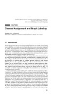
that performs the scheduling of packet transmissions for the cell (see Figure 8.1). Neigh-
boring cells are assumed to transmit on different logical channels. All transmissions are
either uplink (from a mobile host to a base station) or downlink (from a base station to a
mobile host). Each cell has a single logical channel that is shared by all mobile hosts in the
cell. (This discussion also applies to multi-channel cellular networks, under certain re-
strictions.) Every mobile host in a cell can communicate with the base station, though it is
not required for any two mobile hosts to be within range of each other. Each flow of pack-
ets is identified by a <host, uplink/downlink flag, flow id> triple, in addition to other

packet identifiers.
The distinguishing characteristics of the model under consideration are:
ț Channel capacity is dynamically varying
ț Channel errors are location-dependent and bursty in nature [5]
ț There is contention for the channel among multiple mobile hosts
172
FAIR SCHEDULING IN WIRELESS PACKET DATA NETWORKS
ț Mobile hosts do not have global channel status (in terms of which other hosts are
contending for the same channel, etc.)
ț The scheduling must take care of both uplink and downlink flows
ț Mobile hosts are often constrained in terms of processing power and battery power
Thus, any wireless scheduling and channel access algorithm must consider the constraints
imposed by this environment.
In terms of the wireless channel model, we consider a single channel for both uplink
and downlink flows, and for both data and signaling. Even though all the mobiles and the
base station share the same channel, stations may perceive different levels of channel error
patterns due to location-dependent physical layer impairments (e.g., cochannel interfer-
ence, hidden terminals, path loss, fast fading, and shadowing). User mobility also results
in different error characteristics for different users. In addition, it has been shown in [5]
8.2 MODELS AND ISSUES
173
(Scheduler)
Base Station
Mobile 6
<1,Downlink, 0>
Mobile 1
Mobile 4
Mobile 2
<2,Uplink,0>
<3,Uplink,0>

Mobile 3
<4,Downlink,0>
Mobile 5
<5,Downlink,0>
<6,Uplink,0>
<6,Downlink,1>
<3,Downlink,1>
Figure 8.1 Cellular architecture.
that errors in wireless channels occur in bursts of varying lengths. Thus, channel errors are
location-dependent and bursty. This means that different flows perceive different channel
capacities. Note that channel errors result in both data loss and reduce channel capacity.
Although data loss can be addressed using a range of techniques, such as forward error
correction (FEC), the important issue is to address capacity loss, which is the focus of all
wireless fair queueing algorithms.
A flow is said to perceive a clean channel if both the communicating endpoints per-
ceive clean channels and the handshake can take place. A flow is said to perceive a dirty
channel if either endpoint perceives a channel error. We assume a mechanism for the (pos-
sibly imperfect) prediction of channel state. This is reasonable, since typically channel er-
rors, being bursty, are highly correlated between successive slots. Hence, every host can
listen to the base station, and the base station participates in every data transmission by
sending either data or an acknowledgement. Thus, every host that perceives a clean chan-
nel must be able to overhear some packet from the base station during each transmission.
We assume that time is divided into slots, where a slot is the time for one complete
packet transmission including control information. For simplicity of discussion, we con-
sider packets to be of fixed size. However, all wireless fair queueing algorithms can han-
dle variable size packets as well. Following the popular CSMA/CA paradigm [9], we as-
sume that each packet transmission involves a RTS-CTS handshake between the mobile
host and the base station that precedes the data transmission. Successful receipt of a data
packet is followed by an acknowledgement. At most one packet transmission can be in
progress at any time in a cell.

Note that although we use the CSMA/CA paradigm as a specific instance of a wireless
medium access protocol, this is not a requirement in terms of the applicability of the wire-
less fair queueing algorithms described in this chapter. The design of the medium access
protocol is tied very closely to that of the scheduler; however, the issues that need to be
addressed in the medium access protocol do not limit the generality of the issues that need
to be addressed in wireless fair queueing [10, 11]. The design of a medium access protocol
is a subject requiring detailed study and, in this chapter, we will merely restrict our atten-
tion to the impact a scheduling algorithm has on the medium access protocol.
8.2.2 Fluid Fair Queueing
We now provide a brief overview of fluid fair queueing in wireline networks. Consider a
unidirectional link that is being shared by a set F of data flows. Consider also that each
flow f
ʦ
F has a rate weight r
f
. At each time instant t, the rate allocated to a backlogged
flow f is r
f
C(t)/⌺
i
ʦ
B(t)
r
i
, where B(t) is the set of nonempty queues and C(t) is the link ca-
pacity at time t. Therefore, fluid fair queueing serves backlogged flows in proportion to
their rate weights. Specifically, for any time interval [t
1
, t
2

] during which there is no
change in the set of backlogged flows B(t
1
, t
2
), the channel capacity granted to each flow i,
W
i
(t
1
, t
2
), satisfies the following property:
᭙i, j ʦ B(t
1
, t
2
),
Έ
–
Έ
= 0. (8.1)
W
j
(t
1
, t
2
)
ᎏ

r
j
W
i
(t
1
, t
2
)
ᎏ
r
i
174
FAIR SCHEDULING IN WIRELESS PACKET DATA NETWORKS
The above definition of fair queueing is applicable to both channels with constant capaci-
ty and channels with time varying capacity.
Since packet switched networks allocate channel access at the granularity of packets
rather than bits, packetized fair queueing algorithms must approximate the fluid model.
The goal of a packetized fair queueing algorithm is to minimize |W
i
(t
1
, t
2
)/r
i
– W
j
(t
1

, t
2
)/r
j
|
for any two backlogged flows i and j over an arbitrary time window [t
1
, t
2
]. For example,
weighted fair queueing (WFQ) [4] and packet generalized processor sharing (PGPS) [18]
are nonpreemptive packet fair queueing algorithms that simulate fluid fair queueing and
transmit the packet whose last bit would be transmitted earliest according to the fluid fair
queueing model.
In WFQ, each packet is associated with a start tag and finish tag, which correspond re-
spectively to the “virtual time” at which the first bit of the packet and the last bit of the
packet are served in fluid fair queueing. The scheduler then serves the packet with the
minimum finish tag in the system. The kth packet of flow i that arrives at time A( p
i
k
) is al-
located a start tag, S( p
i
k
), and a finish tag, F( p
i
k
), as follows:
S( p
i

k
) = max{V [A( p
i
k
)], F( p
i
k–1
)}
where V(t), the virtual time at time t, denotes the current round of service in the corre-
sponding fluid fair queueing service.
F( p
i
k
) = S( p
i
k
) + L
i
k
/r
i
where L
i
k
is the length of the kth packet of flow i.
The progression of the virtual time V(t) is given by
=
where B(t) is the set of backlogged flows at time t. As a result of simulating fluid fair
queueing, WFQ has the property that the worst-case packet delay of a flow compared to
the fluid service is upper bounded by one packet. A number of optimizations to WFQ, in-

cluding closer approximations to the fluid service and reductions in the computational
complexity, have been proposed in literature (see [22] for an excellent survey).
8.2.3 Service Model for Fairness in Wireless Networks
Wireless fair queueing seeks to provide the same service to flows in a wireless environ-
ment as traditional fair queueing does in wireline environments. This implies providing
bounded delay access to each flow and providing full separation between flows. Specifi-
cally, fluid fair queueing can provide both long-term fairness and instantaneous fairness
among backlogged flows. However, we show in Section 8.2.4 that in the presence of loca-
tion-dependent channel error, the ability to provide both instantaneous and long-term fair-
ness will be violated. Channel utilization can be significantly improved by swapping
channel access between error-prone and error-free flows at any time, or by providing error
C(t)
ᎏ
⌺
i
ʦ
B(t)
r
i
dV(t)
ᎏ
dt
8.2 MODELS AND ISSUES
175
correction (FEC) in the packets. This will provide long-term fairness but not instanta-
neous fairness, even in the fluid model in wireless environments. Since we need to com-
promise on complete separation (the degree to which the service of one flow is unaffected
by the behavior and channel conditions of another flow} between flows in order to im-
prove efficiency, wireless fair queueing necessarily provides a somewhat less stringent
quality of service than wireline fair queueing.

We now define the wireless fair service model that wireless fair queueing algorithms
typically seek to satisfy, and defer the discussion of the different aspects of the service
model to subsequent sections. The wireless fair service model has the following proper-
ties:
ț Short-term fairness among flows that perceive a clean channel and long-term fair-
ness for flows with bounded channel error
ț Delay bounds for packets
ț Short-term throughput bounds for flows with clean channels and long-term through-
put bounds for all flows with bounded channel error
ț Support for both delay-sensitive and error-sensitive data flows
We define the error-free service of a flow as the service that it would have received at
the same time instant if all channels had been error-free, under identical offered loads. A
flow is said to be leading if it has received channel allocation in excess of its error-free
service. A flow is said to be lagging if it has received channel allocation less than its error-
free service. If a flow is neither leading nor lagging, it is said to be “in sync,” since its
channel allocation is exactly the same as its error-free service. If the wireless scheduling
algorithm explicitly simulates the error-free service, then the lead and lag can be easily
computed by computing the difference of the queue size of a flow in the error-free service
and the actual queue size of the flow. If the queue size of a flow in the error-free service is
larger, then the flow is leading. If the queue size of a flow in the error-free service is
smaller, then the flow is lagging. If the two queue sizes are the same, then the flow is in
sync.
8.2.4 Issues in Wireless Fair Queueing
From the description of fair queueing in wireline networks in Section 8.2.2 and the de-
scription of the channel characteristics in Section 8.2.3, it is clear that adapting wireline
fair queueing to the wireless domain is not a trivial exercise. Specifically, wireless fair
queueing must deal with the following issues that are specific to the wireless environment.
ț The failure of traditional wireline fair queueing in the presence of location-depen-
dent channel error.
ț The compensation model for flows that perceive channel error: how transparent

should wireless channel errors be to the user?
ț The trade off between full separation and compensation, and its impact on fairness
of channel access.
176
FAIR SCHEDULING IN WIRELESS PACKET DATA NETWORKS
ț The trade-off between centralized versus distributed scheduling and the impact on
medium access protocols in a wireless cell.
ț Limited knowledge at the base stations about uplink flows: how does the base sta-
tion discover the backlogged state and arrival times of packets at the mobile host?
ț Inaccuracies in monitoring and predicting the channel state, and its impact on the ef-
fectiveness of the compensation model.
We now address all of the issues listed above, except the compensation model for flows
perceiving channel error, which we describe in the next section.
8.2.4.1 Why Wireline Fair Queueing Fails over Wireless Channels
Consider three backlogged flows during the time interval [0, 2] with r
1
= r
2
= r
3
. Flow 1
and flow 2 have error-free channels, whereas flow 3 perceives a channel error during the
time interval [0, 1). By applying equation (1.1) over the time periods [0, 1) and [1, 2], we
arrive at the following channel capacity allocation:
W
1
[0, 1) = W
2
[0,1) =
1

–
2
, W
1
[1, 2] = W
2
[1, 2] = W
3
[1, 2] =
1
–
3
Now, over the time window [0, 2], the allocation is
W
1
[0, 2] = W
2
[0, 2] =
5
–
6
, W
3
[0, 2] =
1
–
3
which does not satisfy the fairness property of equation (8.1). Even if we had assumed
that flow 3 had used forward error correction to overcome the error in the interval [0, 1),
and shared the channel equally with the other two flows, it is evident that its application-

level throughput will be less than that of flows 1 and 2, since flow 3 experiences some ca-
pacity loss in the interval [0, 1). This simple example illustrates the difficulty in defining
fairness in a wireless network, even in an idealized model. In general, due to location-de-
pendent channel errors, server allocations designed to be fair over one time interval may
be inconsistent with fairness over a different time interval, though both time intervals have
the same backlogged set.
In the fluid fair queueing model, when a flow has nothing to transmit during a time
window [t, t + ⌬], it is not allowed to reclaim the channel capacity that would have been
allocated to it during [t, t + ⌬] if it were backlogged at t. However, in a wireless channel, it
may happen that the flow is backlogged but unable to transmit due to channel error. In
such circumstances, should the flow be compensated at a later time? In other words,
should channel error and empty queues be treated the same or differently? In particular,
consider the scenario when flows f
1
and f
2
are both backlogged, but f
1
perceives a channel
error and f
2
perceives a good channel. In this case, f
2
will additionally receive the share of
the channel that would have been granted to f
1
in the error-free case. The question is
whether the fairness model should readjust the service granted to f
1
and f

2
in a future time
window in order to compensate f
1
. The traditional fluid fair queueing model does not need
to address this issue since in a wireline model, either all flows are permitted to transmit or
none of them is.
8.2 MODELS AND ISSUES
177
In order to address this issue, wireless fair queueing algorithms differentiate between a
nonbacklogged flow and a backlogged flow that perceives channel error. A flow that is not
backlogged does not get compensated for lost channel allocation. However, a backlogged
flow f that perceives channel error is compensated in future when it perceives a clean
channel, and this compensation is provided at the expense of those flows that received ad-
ditional channel allocation when f was unable to transmit. Of course, this compensation
model makes channel errors transparent to the user to some extent, but only at the expense
of separation of flows. In order to achieve a trade-off between compensation and separa-
tion, we bound the amount of compensation that a flow can receive at any time. Essential-
ly, wireless fair queueing seeks to make short error bursts transparent to the user so that
long-term throughput guarantees are ensured, but exposes prolonged error bursts to the
user.
8.2.4.2 Separation versus Compensation
Exploring the trade-off between separation and compensation further, we illustrate a typi-
cal scenario and consider several possible compensation schemes. Let flows f
1
, f
2
, and f
3
be three flows with equal weights that share a wireless channel. Let f

1
perceive a channel
error during a time window [0, 1), and during this time window, let f
2
receive all the addi-
tional channel allocation that was scheduled for f
1
(for example, because f
2
has packets to
send at all times, while f
3
has packets to send only at the exact time intervals determined
by its rate). Now, suppose that f
1
perceives a clean channel during [1, 2]. What should the
channel allocation be?
During [0, 1], the channel allocation was as follows:
W
1
[0, 1) = 0, W
2
[0, 1) =
2
–
3
, W
3
[0, 1) =
1

–
3
Thus, f
2
received one-third units of additional channel allocation at the expense of f
1
,
while f
3
received exactly its contracted allocation. During [1, 2], what should the channel
allocation be? In particular, there are two questions that need to be answered:
1. Is it acceptable for f
3
to be impacted due to the fact that f
1
is being compensated
even though f
3
did not receive any additional bandwidth?
2. Over what time period should f
1
be compensated for its loss?
In order to provide separation for flows that receive exactly their contracted channel allo-
cation, flow f
3
should not be impacted at all by the compensation model. In other words,
the compensation should only be between flows that lag their error-free service and flows
that lead that error-free service, where error-free service denotes the service that a flow
would have received if all the channels were error-free.
The second question is how long it takes for a lagging flow to recover from its lag. Of

course, a simple solution is to starve f
2
in [1, 2] and allow f
1
to catch up with the following
allocation:
W
1
[1, 2] =
2
–
3
, W
2
[1, 2] = 0, W
3
[1, 2) =
1
–
3
178
FAIR SCHEDULING IN WIRELESS PACKET DATA NETWORKS
However, this may end up starving flows for long periods of time when a backlogged flow
perceives channel error for a long time. Of course, we can bound the amount of compen-
sation that a flow can receive, but that still does not prevent pathological cases in which a
single backlogged flow among a large set of backlogged flows perceives a clean channel
over a time window, and is then starved out for a long time until all the other lagging flows
catch up. In particular, the compensation model must provide for a graceful degradation of
service for leading flows while they give up their lead.
8.2.4.3 Centralized versus Distributed Scheduling

In a cell, hosts are only guaranteed to be within the range of the base station and not other
hosts, and all transmissions are either uplink or downlink. Thus, the base station is the
only logical choice for the scheduling entity in a cell, making the scheduling centralized.
However, although the base station has full knowledge of the current state of each down-
link flow (i.e., whether it is backlogged, and the arrival times of the packets), it has limited
and imperfect knowledge of the current state of each uplink flow. In a centralized ap-
proach, the base station has to rely on the mobile hosts to convey uplink state information
for scheduling purposes, which adds to control overhead for the underlying medium ac-
cess protocol.
In a distributed approach, every host with some backlogged flows (including the base
station) will have imperfect knowledge of other hosts’ flows. Thus, the medium access
protocol will also have to be decentralized, and the MAC must have a notion of priority
for accessing the channel based on the eligibility of the packets in the flow queues at
that host (e.g., backoffs). Since the base station does not have exclusive control over the
scheduling mechanism, imprecise information sharing among backlogged uplink and
downlink flows will result in poor fairness properties, both in the short term and in the
long term.
In our network model, since the base station is involved in every flow, a centralized
scheduler gives better fairness guarantees than a distributed scheduler. All wireless fair
scheduling algorithms designed for cellular networks follow this model. Distributed
schedulers, however, are applicable in different network scenarios, as will be discussed in
Section 8.5. The important principle here is that the design of the medium access control
(MAC) protocol is closely tied to the type of scheduler chosen.
8.2.4.4 Incomplete State at the Base Station for Uplink Scheduling
When the base station is the choice for the centralized scheduler, it has to obtain the state
of all uplink flows to ensure fairness for such flows. As discussed above, it is impossible
for the centralized scheduler to have perfect knowledge of the current state for every up-
link flow. In particular, the base station may not know precisely when a previously non-
backlogged flow becomes backlogged, and the precise arrival times of uplink packets in
this case. The lack of such knowledge has an impact on the accuracy of scheduling and de-

lay guarantees that can be provided in wireless fair queueing.
This problem can be alleviated in part by piggybacking flow state on uplink transmis-
sions, but newly backlogged flows may still not be able to convey their state to the base
station. For a backlogged flow, the base station only needs to know if the flow will contin-
ue to remain backlogged even after it is allocated to a channel. This information can be
8.2 MODELS AND ISSUES
179