Tài liệu Mạng lưới giao thông và đánh giá hiệu suất P12 pptx

12
LONG-RANGE DEPENDENCE AND
QUEUEING EFFECTS FOR VBR VIDEO
D
ANIEL
P. H
EYMAN
AT&T Labs, Middletown, NJ 07748
T. V. L
AKSHMAN
Bell Laboratories, Holmdel, NJ 07733
12.1 INTRODUCTION
In this chapter we present some of our results concerningsource models for H.261
coded VBR (variable bit rate) video. Video services have been forecasted to be a
substantial portion of the traf®c on emerging broadband digital networks. Statistical
source models of video traf®c are needed to design networks that delivery acceptable
picture quality at minimum cost, and to control and shape the output rate of the
coder. For example, one issue is decidingwhether a new video connection can be
admitted to a network, and the consequent determination of the bandwidth that must
be allocated to the connection to ensure adequate quality of service. A model of the
bandwidth that the connection will try to consume is required for this task. In
addition to providinga good description of the bandwidth requirements, the source
model should be usable in the connection-acceptance decision model.
Other chapters that contain related material are Chapters 9, 13, 16, and 17.
12.1.1 Special Propertiesof Video
There are some physical reasons why traces from video sources are special. Video is
a succession of regularly spaced still pictures, called frames. Each still picture is
represented in digital form by a coding algorithm, and then compressed to save
Self-Similar NetworkTraf®c and Performance Evaluation, Edited by KihongPark and Walter Willinger
ISBN 0-471-31974-0 Copyright # 2000 by John Wiley & Sons, Inc.
285

Self-Similar NetworkTraf®c and Performance Evaluation, Edited by KihongPark and Walter Willinger
Copyright # 2000 by John Wiley & Sons, Inc.
Print ISBN 0-471-31974-0 Electronic ISBN 0-471-20644-X
bandwidth. See, for example, Netravili and Haskell [24] for full information about
video coding. A common way to save bandwidth is to send a reference frame, and
then send the differences of successive frames. This is called interframe coding.
Since the adjacent pictures cannot be too different from each other (because most
motion is continuous), this generates substantial autocorrelation in the sizes of
frames that are near to each other. To protect against transmission errors, a full frame
is sent periodically. Furthermore, when there is a scene change the frames no longer
depend on the past frames, so functional correlation ends; this may also end the
statistical correlation in the frame sizes. Scene changes require that a complete new
picture be transmitted, so the scene lengths have an effect on the trace. For these and
several other reasons that are too dif®cult to describe here, video traf®c is different
from broadband data traf®c, and so the models and conclusions described in this
chapter may not apply to other types of traf®c.
Video quality degrades when information is lost during transmission or when the
interarrival times of frames are either large or very variable. The latter is controlled
by limitingbuffer sizes; frames that arrive late might as well not arrive at all. Video
engineers often describe the size of a buffer by the length of time it takes to empty it
(which is the maximum delay a frame can incur). Current design objectives are for
a maximum delay of between 100 and 200 ms. Since several buffers may be
encountered from source to destination and there are other sources of delay (e.g.,
propagation time), some studies use 10 ms as the maximum buffer size.
Frames are transmitted in ®xed size units that we call cells. The rate of
information loss is the cell-loss rate or CLR. We are interested in situations where
the cell losses occur because of buffer over¯ow. We consider models of a single
station, where the buffer size and buffer drain rate are given. Under these conditions,
the CLR is controlled by keepingthe traf®c intensity small enough to achieve a
performance goal. A typical performance goal is to keep the CLR no larger than

10
Àk
, where k is usually between three and six.
These contraints on buffer size and CLR (and indirectly on traf®c intensity) give
rise to a practical region of operation where the constraints are satis®ed. The notion
of ``high'' traf®c intensity is related to these constraints. When the design parameters
(e.g., buffer size and processing speed) are speci®ed, the traf®c intensity is high
when the constraints are just barely satis®ed.
12.1.2 Source Modeling
The central problem of source modelingis to choose how to represent data traces by
statistical models. A source model is sought for a purpose, which is usually as an
input process to a performance model. We think that a source model is acceptable if
it ``adequately'' describes the trace in the performance model at hand. By adequate
we mean that when the source model is used in the performance model, the values of
the operatingcharacteristics of interest produced are ``close enough'' to the value
produced by the trace. The de®nition of close enough may depend on the use to
which the performance model will be put. For example, long-range network
286
LONG-RANGE DEPENDENCE AND QUEUEING EFFECTS FOR VBR VIDEO
planningtypically requires less accuracy for delay statistics and loss rates than
equipment engineering does.
We don't regard good source models for a given trace to be unique. Different
purposes may best be served by different models. For example, the DAR and GBAR
models described in Sections 12.2.2 and 12.2.3 are designed for different purposes.
A consequence of our emphasis on testingsource models by how well they emulate
the behavior of the trace they model in a performance model is that the con®dence
intervals we emphasize are on the operatingcharacteristics of the performance
models.
12.1.3 Outine
We divide VBR video into two classes, video conferences and entertainment video.

Section 12.2 contains two models for video conferences, and Section 12.3 contains a
model for entertainment video. The models are vetted by comparingthe performance
measures they induce in a simulation to the performance measures induced by data
traces. All of these models are Markov chains, so they are short-range dependent
(SRD). Hurst parameter estimates for the time series these models describe indicate
the presence of long-range dependence. The reasons that short-range dependent
models can provide good models for time series that exhibit long-range dependence
are given in detail in Section 1.4. Our results are summarized in the last section.
12.2 VIDEO CONFERENCES
Video conferences show talkingheads and may be the easiest type of video to
model. The models developed for them will be expanded to describe entertainment
video in Section 1.3.
12.2.1 Source Data
We have data from three different coders and four video teleconferences of about
one-half hour in length. The data consists of the size of each still picture, that is, of
each frame. All of the teleconferences show a head-and-shoulders scene with
moderate motion and scene changes, and with little camera zoom or pan. All of
the coders use a version of the H.261 video codingstandard. The key differences in
the sequences are that sequence A was recorded by a coder that uses neither discrete-
cosine transform (DCT) nor motion compensation, sequence B was recorded by a
coder that uses both DCT and motion compensation, and sequences C and D were
recorded by a coder that used DCT but not motion compensation. The graphs in
Figs. 12.1 and 12.2 show that the details (presence or absence of DCT or motion
compensation) do not have a signi®cant effect on the statistics of interest to us here.
The summary statistics of these sequences are given in Table 12.1.
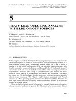
All of these sequences are adequately described by negative-binomial marginal
distributions and geometric autocorrelation functions. Figure 12.1 shows Q-Q plots
of the marginal distributions, which have been divided by their means; the ®t is
12.2 VIDEO CONFERENCES
287

D ATA
gamma
Fig. 12.1 Q-Q plots for four sequences.
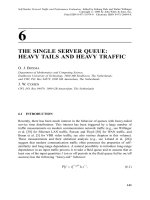
Autocorrelation function
Lag (frames)
Fig. 12.2 Autocorrelation functions.
288
LONG-RANGE DEPENDENCE AND QUEUEING EFFECTS FOR VBR VIDEO
excellent for sequences C and D, good for sequence A, and adequate for sequence B.
The negative-binomial distribution is the discrete analog of the gamma distribution,
and a discretized version of the latter can be used when it is more convenient to
do so.
Figure 12.2 shows the autocorrelation functions. The ordinate has a log scale, so
geometric functions will appear as straight lines. The geometric property holds for at
least 100 lags (2.5 seconds) for sequences B, C, and D, and for 50 lags for sequence
A. For lags larger than 250, the geometric function underestimates the autocorrela-
tion function. We examined sequences A, B, and C and concluded they possess long-
range dependence. Since the autocorrelation functions shown in Fig. 12.2 are so
large for small lags, it seem intuitive (to us, at least) that the short-range correlations
should be the important ones to capture in a source model. We propose usingthe
geometric function r
k
for the autocorrelation function.
Since the negative-binomial and gamma distributions are speci®ed by two
parameters, these parameters can easily be esimated from the mean and the variance
of the number of cells per frame by the method of moments. Only those two
moments and the correlation coef®cient (r) are needed to specify the key properties
of VBR teleconference traf®c. The correlation coef®cient can be estimated from the
geometric portion of the autocorrelation function by taking logarithms and doing a
linear regression.

12.2.2 The DAR Model
Our ®rst investigations of these sequences with Tabatabai [16] and Heeke [18]
focused on multiplexingissues. First, we established that the time series were
stationary. This was done by examiningplots of smoothed versions of the time series
and boxplots of many partitions of the time series. Next, we showed a Markov chain
provided a good description of the time series. This was done via simulations as
described in Section 12.2.2.1. This means that the marginal distributions of the time
series can be viewed as the steady-state distributions of the Markov chain. A Markov
chain that has a geometric autocorrelation function and whose steady-state distribu-
tion can be speci®ed is the DAR(1) process introduced by Jacobs and Lewis [20].
The only member of the DARk family that is used here is the DAR(1), so the (1)
will be deleted. The transition matrix is given by
P  rI 1 À rQ; 12:1
TABLE 12.1 Summary Statistics of Data Sequences
Sequence Bytes per Cell Mean (cells) Standard Deviation (cells) r
A 14 1506.4 512.7 0.981
B 48 104.9 29.7 0.984
C 64 130.3 74.4 0.985
D 64 170.6 107.6 0.970
12.2 VIDEO CONFERENCES
289
where r is the lag-one autocorrelation coef®cient. I is the identity matrix, and each
row of Q consists of the steady-state probabilities. In our case the steady-state
probabilities are the negative-binomial probabilities described above, truncated at
some convenient value at least as large as the peak rate (the missing probability is
added to the last probability kept).
Equation (12.1) is convenient for analytical work, but it masks the simplicity of
the DAR model. Let X
n
be the size (in bits, bytes, or cells as appropriate) of the nth

frame and r be as above; the DAR model is
X
n

X
nÀ1
with probability r;
X
H
with probability 1 À r;

12:2
where X
H
is a sample from the marginal distribution (negative-binomial in our case).
From Eq. (12.2) we see that the X -process maintains a constant value (cell rate) for a
geometrically distributed number of steps (frames) with mean 1=1 À r, and then
another value (possibly the same as the old value) is chosen. When r is close to one
(it is about 0.98 in our examples, see Table 12.1), the mean time between cell rate
changes is large (about 50 frames in our examples). This means that the sample
paths are constant for longintervals. The data trace doesn't have this property, which
is the reason the GBAR model described in Section 12.2.3 was introduced. This
difference between the sample paths of the model and the data trace is mitigated
when several sources are multplexed. The probability that X
H
n
 X
nÀ1
is small
enough to be ignored in the following calculation. When k sources are multiplexed,

X
n
 X
n
À 1 with probability r
k
, so the mean time between potential cell rate
changes with r  0:98 and k  16 is 3.6. Consequently, sample paths of the
multiplexed cell streams from 16 sources are not constant for longintervals.
12.2.2.1 Validating the DAR Model We validate the DAR model by lookingat
performance models for multplexinggain and connection admission control. To
estimate statistical multiplexinggain, we use cell-loss probabilities [16] from a
simple model of a switch. The source model is a FIFO buffer that is drained at
45 Mb=s. The length of the buffer is expressed as the time to drain a full buffer; this
is the maximum possible delay. The results of ten simulations of the DAR model for
sequence C are given by 95% con®dence intervals and are shown in Table 12.2. The
TABLE 12.2 Cell-Loss Rates for Trace and 95% Con®dence Intervals for DAR Model
of Sequence C
Buffer Size (ms)
Source 1 2 3 4 5
Probability of Loss Â10
À6
for Various Buffer Sizes
Trace 2070.0 527.0 141.0 33.3 2.88
DAR model (1738, 2762) (433, 775) (107.4, 212.6) (15.1, 54.1) (2.26, 9.34)
290
LONG-RANGE DEPENDENCE AND QUEUEING EFFECTS FOR VBR VIDEO
results of these simulations show that the DAR model does a good job of estimating
the cell-loss rate when 16 sources are multiplexed. Similar results were obtained for
the other sequences [18].

Now we consider connection admission control (CAC). Since the DAR model is a
Markov chain model of the source, it conforms to one of the sets of conditions a
source model must have for the effective bandwidth (EBW) theory of Elwalid and
Mitra [8]. Moreover, the DAR model is a reversible Markov chain, and so it inspired
a powerful extension of the EBW method, called the Chernoff-dominated eigenvalue
(CCE) method [7]. Suppose we have a switch that can process at rate C (Mb=s) and
has a buffer of size B (ms). We want to ®nd the maximum number of statistically
homogeneous sources that can be admitted while keeping the cell-loss rate no larger
than 10
À6
. The CDE method gives an approximate analytic solution with known
error bounds; this solution is denoted by K
CDE
. Another way to obtain the solution is
to test candidate values by evaluatingthe cell-loss rate by simulation; we treat this as
the exact solution and denote it by K
sim
. Table 12.3 compares the results of the CDE
method to the CAC found from simulations. The number admitted by the CDE
method is a very close approximation to the ``true'' value obtained by simulation.
This implies that the DAR model captures enough of the statistical properties of the
trace to produce good admission decisions.
12.2.3 The GBAR Model
The DAR model may not be suitable for a single source (by a single source we mean
a source that does not interact with other sources) as described above. Lucantoni et
al. [22] give three areas where single source models are useful: studying what types
of traf®c descriptors make sense for parameter negotiation with the network at call
setup, testing rate control algorithms, and predicting the quality of service degrada-
tion caused by congestion on an access link. For this reason, Heyman [11] proposed
the GBAR model. Lakshman et al. [21] use the GBAR model to predict frame sizes

in a rate control algorithm.
Lucantoni et al. [22] propose a Markov-renewal process model to describe a
single source. This model has the advantage of being very general, and the
disadvantage that it is not parameterized by some simple summary statistics of the
data trace. The GBAR model exploits the properties enjoyed by teleconferencing
traf®c described in Section 12.2.2, the geometrically decaying autocorrelation
TABLE 12.3 CAC Performance for Video Conference A and Video Conference C
Video Conference A Video Conference B
B 57 9 50 44 5 0.5 9 23 7 1 8.5 9.5 10 11
C 45 67 81 103 125 145 195 245 270 310 110 185 280 375
K
sim
20 30 40 50 60 70 98 128 139 156 16 30 49 66
K
CDE
16 25 33 44 53 63 90 120 130 150 15 30 50 70
12.2 VIDEO CONFERENCES
291
function and the negative-binomial (or gamma) marginal distributions, to produce a
simple model based on the three parameters that describe these features.
The GBAR(1) process was introduced by McKenzie [23], alongwith some other
interestingautoregressive processes. (As with the DAR model we will drop the
argument (1).) Two inherent features of this process are the marginal distribution is
gamma and the autocorrelation function is geometric.
Toward de®ningthe GBAR model, let Gab; l denote a random variable with a
gamma distribution with shape parameter b and scale parameter l; that is, the
density function is
f
G
t

llt
b
Gb  1
e
Àlt
; t > 0: 12:3
Similarly, let Bep; q denote a random variable with a beta distribution with
parameters p and q; that is, with density function
f
B
t
G p  q
G p  1Gq  1
t
p
1 À t
q
; 0 < t < 1; 12:4
where p and q are both larger than À1. The GBAR model is based on two well-
known results: the sum of independent Gaa; l and Gab; l random variables is a
Gaa  b; l random variable, and the product of independent Bea; b À a and
Gab; l random variables is a Gaa; l random variable. Thus, if X
nÀ1
is Gab; l,
A
n
is Bea; b À a, and B
n
is Gab À a; l, and these three are mutually independent,
then

X
n
 A
n
X
nÀ1
 B
n
12:5
de®nes a stationary stochastic process X
n
with a marginal Gab; l distribution.
Furthermore, the autocorrelation function of this process is given by
rk
a
b

k
; k  0; 1; 2; ... 12:6
The process de®ned by Eq. (12.5) is called the GBAR processes. The G and B
denote gamma and beta, respectively, and the AR stands for autoregressive. Since
the current value is determined by only one previous value, this is an autoregressive
process of order one.
A possible physical interpretation of Eq. (12.5) is the following. Interpret A
n
as
the fraction of frame n À 1 that is used in the predictor of frame n, so the ®rst term
on the left of Eq. (12.5) is the contribution of interframe prediction. In hybrid
PCM=DPCM coding[24], for example, resistance to transmission error is accom-
plished by periodically settingsome differential predictor coef®cients to zero and

sendinga PCM value. We can think of B
n
as the number of cells to do that. If the
292
LONG-RANGE DEPENDENCE AND QUEUEING EFFECTS FOR VBR VIDEO
distributional and independence assumptions listed above Eq. (12.5) are valid, then
the GBAR process will be formed.
Simulatingthe GBAR process only requires the ability to simulate independent
and identically distributed gamma and beta random variables. This is easily done; for
example, algorithms and Fortran programs are presented in Bratley et al. [3].
The GBAR process is used as a source model by generating noninteger values
from Eq. (12.5) and then roundingto the nearest integer. It would be cleaner if a
discrete process with negative-binomial marginals could be generated in the ®rst
place. McKenzie describes such a process (his Eq. (3.6)). Unfortunately, that process
requires much more computation to simulate, and the extra effort does not appear to
be worthwhile.
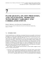
12.2.3.1 Validating the GBAR Model Ten sample paths of the GBAR process
were generated and used as the arrival process (number of cells per frame with a
®xed interframe time) in a simulation of a service system with a ®nite buffer and
a constant-rate server. The cell-loss rates from these paths were averaged to obtain a
point estimate for the GBAR model. The traf®c intensity is varied by changing the
service rate. The points produced by the simulations are denoted by an asterisk. In
Fig. 12.3, we see that cell-loss rates computed from the GBAR model are close to the
cell-loss rates computed from the data. Note that for each traf®c intensity,
the decrease in the cell-loss rate as the buffer size increases is very slight, for
both the model and the data. This con®rms the prediction of Hwangand Li [19] of
buffer ineffectiveness. Since the GBAR model has only short-range dependence, this
effect is not caused by long-range dependence here.
B()
Fig. 12.3 Cell-loss rates for sequence A.

12.2 VIDEO CONFERENCES
293
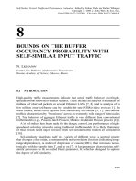
Figure 12.4 shows that the mean queue lengths in an in®nite buffer computed
from ®ve GBAR paths are similar to the mean queue lengths computed using the
data. In Fig. 12.4 the vertical axis on the left shows the mean queue length in cells.
Video quality is poor when the cell delays are large; 100 ms is an upper bound on the
acceptable delay at a node in a network that provides video services. Two buffer
drain times are also shown; the practical region for the maximum is below and to the
left of the 100 ms line. The range of the mean queue lengths shown exceeds the
practical region for maximum queue length. In the practical region, the model and
the trace give very similar mean delays. The differences between the mean queue
length from the GBAR model and the mean queue lengths from the data would be
even smaller if a ®nite buffer were imposed. (This is the truncatingeffects of ®nite
buffers that is described in Section 12.4.2). The comparisons for sequences B, C, and
D are qualitatively the same as for sequence A.
12.3 BROADCAST VIDEO
Now we turn to more dynamic sequences, such as ®lms, news, sports, and
entertainment television. Since the main purpose of the models is to aid in network
performance evaluations, we are particularly interested in usingthe models to predict
cell-loss rates.
T
M
()
Fig. 12.4 Mean queue lengths for sequence A.
294
LONG-RANGE DEPENDENCE AND QUEUEING EFFECTS FOR VBR VIDEO
Broadcast VBR-coded video has different bit-rate characteristics than VBR-
coded video conferences. Video conference sequences consist of head-and-shoulders
pictures with little or no panning, while broadcast video is characterized by a
succession of scenes. With interframe coding, it is clear that scene changes require

more bits than intrascene frames, so broadcast video will differ from video
conferences in at least this respect; this was demonstrated by Yasuda et al. [32].
There are some other differences too, as demonstrated by Verbiest et al. [31] and
further ampli®ed by Verbiest and Pinnoo [30]. In these papers, a DPCM-based
codingalgorithm is used. In the latter paper, it is shown that the number of bits per
frame has a different autocorrelation function for broadcast video than for video
conferences or video telephony. The autocorrelation functions for the last two are
similar to each other and decay geometrically to zero. For broadcast video, the
autocorrelation function does not decay to zero. Moreover, the ®rst frame after a
scene change has signi®cantly more bits than other frames in the scene. Ramamurthy
and Sengupta [26] observe that the correlation function declines more rapidly at
small lags than at large lags, and that the time series can be described by a semi-
Markov process that has states identi®ed by the bit rates for different types of scenes
(and a state for scene changes). We build on this idea [12]; the simple DAR and
GBAR models that described video conferences are not suf®cient for broadcast
video, although the DAR model is used as a building block in a more complex
model.
12.3.1 Modeling Broadcast Video
We obtained several data sets giving the number of bits per frame for sequences
encoded by an intra®eld=interframe DPCM codingscheme without use of DCT or
motion compensation. We did not have access to the actual video sequences. Hence,
a visual identi®cation of scene-change frames was not possible. Our modeling
strategy was to ®rst develop a way to identify scene changes, then construct models
for the lengths of the scenes and the number of cells in a scene-change frame.
Finally, models for the number of cells per frame for frames within scenes were
developed.
12.3.1.1 Preliminary Data Analysis Before describingthe statistical models, we
report some elementary statistics about the sequences we examined. Figure 12.5
shows the peak and mean bit rates, and their ratios.
The peak-to-mean ratios vary from 1.3 to 2.4. By way of comparision, the peak-

to-mean ratio for video-conference sequence with this codec (sequence A) is 3.2.
Note that the larger peak-to-mean ratios are associated with the lower mean bit rates.
The sequences divers, ®lm, Isuara 1, and Isaura 2, which have a low mean rate and
high peak-to-mean ratios, were different TV programs recorded from a Cable TV
network (and designated as normal quality broadcast video). The sequences with low
peak-to-mean ratios (such as football, sport, news, etc.) were taken directly from the
TV studios (and designated high-quality broadcast video).
12.3 BROADCAST VIDEO
295
12.3.2 Identifying Scene Changes
Figure 12.6 shows two segments of the trace of ®lm, and it can be seen that there are
several spikes that are possibly due to scene changes. Since these spikes may be a
dominant cause of cell losses, we need to model both their spacingand the
magnitude. If we use merely ®xed spacing at the correct rate but do not model
the distribution of their spacing, multiplexed sources with nonidentical starting
points will not have coincident spikes from time to time. This will underestimate cell
losses.
Since we do not have a video record of the sequences, we will assume that a scene
change occurs when a frame contains an abnormally large number of cells compared
to its neighbors. We make this notion quantitative in the following way. Let X
i
be
the number of cells in frame i. At a scene change, the second difference
X
i1
À X
i
ÀX
i
À X

iÀ1
 will be large in magnitude and negative in sign. To
quantify what we mean by large, we divide the second difference by the average
of the past few frames. We found that using25 frames (1 second) in the average was
about the same as using6 frames (about
1
4
second), and the latter was adopted. We
chose À0:5 as the critical value; this choice is entirely subjective. It would be nice if
the subjectivity could be replaced by an objective criterion. We examined the
statistical theory of outlier identi®cation for guidance and concluded that this is
wishful thinkingbecause objective tests need to have ``outlier'' speci®ed externally.
To see if our criterion identi®ed scene changes accurately, we looked at the time
series X
i
and the correspondingvalues of the scaled second differences. Some of the
M/
P
Isaura 2
Isaura 1
Fig. 12.5 Peak-to-mean ratios.
296
LONG-RANGE DEPENDENCE AND QUEUEING EFFECTS FOR VBR VIDEO
data are shown in Fig. 12.6. The ®rst 1000 frames are shown on the left. The test
values identify the scene changes with no false positives. The choice of À0:5 as the
critical value is not signi®cant. Frames 9001 through 10,000 are shown on the right.
This is a more active (in terms of bit-rate ¯uctuations) subsequence, and changing
the critical value will affect the number of frames identi®ed as scene changes. There
are 317 scene changes when À0:5 is the critical value (the mean scene length is 6.5
seconds); there are 374 when À0:4 is used, and 283 when À0:6 is used. The density

functions of the scene lengths produced by these critical values are shown in Fig.
12.7. We observe that the critical value does not have a large effect on the density
function.
12.3.2.1 Scene Lengths Plots of the autocorrelation function showed that scene
lengths are uncorrelated, so the main modeling issue is to characterize the distribu-
tion of the number of frames in a scene. The shape of the density in Fig. 12.7 was
observed on all sequences except for news. (This is a news broadcast. There are 134
scene changes, and 75 of them are 3 frames long. Moreover, most of these occur
consecutively. We do not have an explanation for this. The 3-frame scenes were
deleted and the remainder are called news.d.)
This unimodal and long-tailed shape is characteristic of distributions used in
reliability and insurance-loss models. We will use the followingthree distributions as
candidates for describingscene lengths (and the number of cells per frame in the
sequel).
Fig. 12.6 Bit rates and scaled second differences.
12.3 BROADCAST VIDEO
297