Tài liệu Ten Principles of Economics - Part 15 ppt

CHAPTER 7 CONSUMERS, PRODUCERS, AND THE EFFICIENCY OF MARKETS 147
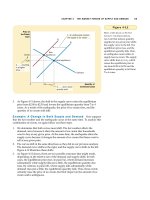
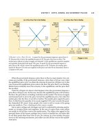
Now suppose that the price falls from P
1
to P
2
, as shown in panel (b). The con-
sumer surplus now equals area ADF. The increase in consumer surplus attribut-
able to the lower price is the area BCFD.
This increase in consumer surplus is composed of two parts. First, those buy-
ers who were already buying Q
1
of the good at the higher price P
1
are better off be-
cause they now pay less. The increase in consumer surplus of existing buyers is the
reduction in the amount they pay; it equals the area of the rectangle BCED. Sec-
ond, some new buyers enter the market because they are now willing to buy the
good at the lower price. As a result, the quantity demanded in the market increases
from Q
1
to Q
2
. The consumer surplus these newcomers receive is the area of the tri-
angle CEF.
WHAT DOES CONSUMER SURPLUS MEASURE?
Our goal in developing the concept of consumer surplus is to make normative
judgments about the desirability of market outcomes. Now that you have seen
what consumer surplus is, let’s consider whether it is a good measure of economic
well-being.
Imagine that you are a policymaker trying to design a good economic system.
Would you care about the amount of consumer surplus? Consumer surplus, the

amount that buyers are willing to pay for a good minus the amount they actually
pay for it, measures the benefit that buyers receive from a good as the buyers them-
selves perceive it. Thus, consumer surplus is a good measure of economic well-being
if policymakers want to respect the preferences of buyers.
In some circumstances, policymakers might choose not to care about con-
sumer surplus because they do not respect the preferences that drive buyer be-
havior. For example, drug addicts are willing to pay a high price for heroin. Yet we
would not say that addicts get a large benefit from being able to buy heroin at a
low price (even though addicts might say they do). From the standpoint of society,
willingness to pay in this instance is not a good measure of the buyers’ benefit, and
consumer surplus is not a good measure of economic well-being, because addicts
are not looking after their own best interests.
In most markets, however, consumer surplus does reflect economic well-
being. Economists normally presume that buyers are rational when they make de-
cisions and that their preferences should be respected. In this case, consumers are
the best judges of how much benefit they receive from the goods they buy.
QUICK QUIZ: Draw a demand curve for turkey. In your diagram, show a
price of turkey and the consumer surplus that results from that price. Explain
in words what this consumer surplus measures.
PRODUCER SURPLUS
We now turn to the other side of the market and consider the benefits sellers re-
ceive from participating in a market. As you will see, our analysis of sellers’ wel-
fare is similar to our analysis of buyers’ welfare.
148 PART THREE SUPPLY AND DEMAND II: MARKETS AND WELFARE
COST AND THE WILLINGNESS TO SELL
Imagine now that you are a homeowner, and you need to get your house painted.
You turn to four sellers of painting services: Mary, Frida, Georgia, and Grandma.
Each painter is willing to do the work for you if the price is right. You decide to
take bids from the four painters and auction off the job to the painter who will do
the work for the lowest price.

Each painter is willing to take the job if the price she would receive exceeds
her cost of doing the work. Here the term cost should be interpreted as the
painters’ opportunity cost: It includes the painters’ out-of-pocket expenses (for
paint, brushes, and so on) as well as the value that the painters place on their own
time. Table 7-3 shows each painter’s cost. Because a painter’s cost is the lowest
price she would accept for her work, cost is a measure of her willingness to sell her
services. Each painter would be eager to sell her services at a price greater than her
cost, would refuse to sell her services at a price less than her cost, and would be in-
different about selling her services at a price exactly equal to her cost.
When you take bids from the painters, the price might start off high, but it
quickly falls as the painters compete for the job. Once Grandma has bid $600 (or
slightly less), she is the sole remaining bidder. Grandma is happy to do the job for
this price, because her cost is only $500. Mary, Frida, and Georgia are unwilling to
do the job for less than $600. Note that the job goes to the painter who can do the
work at the lowest cost.
What benefit does Grandma receive from getting the job? Because she is will-
ing to do the work for $500 but gets $600 for doing it, we say that she receives pro-
ducer surplus of $100. Producer surplus is the amount a seller is paid minus the
cost of production. Producer surplus measures the benefit to sellers of participat-
ing in a market.
Now consider a somewhat different example. Suppose that you have two
houses that need painting. Again, you auction off the jobs to the four painters. To
keep things simple, let’s assume that no painter is able to paint both houses and
that you will pay the same amount to paint each house. Therefore, the price falls
until two painters are left.
In this case, the bidding stops when Georgia and Grandma each offer to do
the job for a price of $800 (or slightly less). At this price, Georgia and Grandma
are willing to do the work, and Mary and Frida are not willing to bid a lower
price. At a price of $800, Grandma receives producer surplus of $300, and Georgia
receives producer surplus of $200. The total producer surplus in the market

is $500.
Table 7-3
T
HE
C
OSTS OF
F
OUR
P
OSSIBLE
S
ELLERS
S
ELLER
C
OST
Mary $900
Frida 800
Georgia 600
Grandma 500
cost
the value of everything a seller must
give up to produce a good
producer surplus
the amount a seller is paid for a good
minus the seller’s cost
CHAPTER 7 CONSUMERS, PRODUCERS, AND THE EFFICIENCY OF MARKETS 149
USING THE SUPPLY CURVE TO MEASURE
PRODUCER SURPLUS
Just as consumer surplus is closely related to the demand curve, producer surplus

is closely related to the supply curve. To see how, let’s continue our example.
We begin by using the costs of the four painters to find the supply schedule for
painting services. Table 7-4 shows the supply schedule that corresponds to the
costs in Table 7-3. If the price is below $500, none of the four painters is willing to
do the job, so the quantity supplied is zero. If the price is between $500 and $600,
only Grandma is willing to do the job, so the quantity supplied is 1. If the price is
between $600 and $800, Grandma and Georgia are willing to do the job, so the
quantity supplied is 2, and so on. Thus, the supply schedule is derived from the
costs of the four painters.
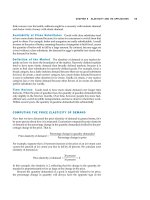
Figure 7-4 graphs the supply curve that corresponds to this supply schedule.
Note that the height of the supply curve is related to the sellers’ costs. At any quan-
tity, the price given by the supply curve shows the cost of the marginal seller, the
Table 7-4
T
HE
S
UPPLY
S
CHEDULE FOR THE
S
ELLERS IN
T
ABLE
7-3
P
RICE
S
ELLERS
Q
UANTITY

S
UPPLIED
$900 or more Mary, Frida, Georgia, Grandma 4
$800 to $900 Frida, Georgia, Grandma 3
$600 to $800 Georgia, Grandma 2
$500 to $600 Grandma 1
Less than $500 None 0
Price of
House
Painting
500
800
$900
0
Quantity of
Houses Painted
600
1234
Supply
Mary’s cost
Frida’s cost
Georgia’s cost
Grandma’s cost
Figure 7-4
T
HE
S
UPPLY
C
URVE

. This figure
graphs the supply curve from the
supply schedule in Table 7-4.
Note that the height of the supply
curve reflects sellers’ costs.
150 PART THREE SUPPLY AND DEMAND II: MARKETS AND WELFARE
seller who would leave the market first if the price were any lower. At a quantity
of 4 houses, for instance, the supply curve has a height of $900, the cost that Mary
(the marginal seller) incurs to provide her painting services. At a quantity of
3 houses, the supply curve has a height of $800, the cost that Frida (who is now the
marginal seller) incurs.
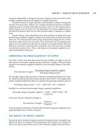
Because the supply curve reflects sellers’ costs, we can use it to measure pro-
ducer surplus. Figure 7-5 uses the supply curve to compute producer surplus in
our example. In panel (a), we assume that the price is $600. In this case, the quan-
tity supplied is 1. Note that the area below the price and above the supply curve
equals $100. This amount is exactly the producer surplus we computed earlier for
Grandma.
Panel (b) of Figure 7-5 shows producer surplus at a price of $800. In this case,
the area below the price and above the supply curve equals the total area of the
two rectangles. This area equals $500, the producer surplus we computed earlier
for Georgia and Grandma when two houses needed painting.
The lesson from this example applies to all supply curves: The area below the
price and above the supply curve measures the producer surplus in a market. The logic is
straightforward: The height of the supply curve measures sellers’ costs, and the
difference between the price and the cost of production is each seller’s producer
surplus. Thus, the total area is the sum of the producer surplus of all sellers.
Quantity of
Houses Painted
Quantity of
Houses Painted

Price of
House
Painting
500
800
$900
0
Supply
600
1234
(b) Price = $800
Price of
House
Painting
500
800
$900
0
600
1234
(a) Price = $600
Supply
Grandma’s producer
surplus ($100)
Georgia’s producer
surplus ($200)
Grandma’s producer
surplus ($300)
Total
producer

surplus ($500)
Figure 7-5
M
EASURING
P
RODUCER
S
URPLUS WITH THE
S
UPPLY
C
URVE
. In panel (a), the price of the
good is $600, and the producer surplus is $100. In panel (b), the price of the good is $800,
and the producer surplus is $500.
CHAPTER 7 CONSUMERS, PRODUCERS, AND THE EFFICIENCY OF MARKETS 151
HOW A HIGHER PRICE RAISES PRODUCER SURPLUS
You will not be surprised to hear that sellers always want to receive a higher price
for the goods they sell. But how much does sellers’ well-being rise in response to
a higher price? The concept of producer surplus offers a precise answer to this
question.
Figure 7-6 shows a typical upward-sloping supply curve. Even though this
supply curve differs in shape from the steplike supply curves in the previous fig-
ure, we measure producer surplus in the same way: Producer surplus is the area
below the price and above the supply curve. In panel (a), the price is P
1
, and pro-
ducer surplus is the area of triangle ABC.
Panel (b) shows what happens when the price rises from P
1

to P
2
. Producer
surplus now equals area ADF. This increase in producer surplus has two parts.
First, those sellers who were already selling Q
1
of the good at the lower price P
1
are
better off because they now get more for what they sell. The increase in producer
surplus for existing sellers equals the area of the rectangle BCED. Second, some
new sellers enter the market because they are now willing to produce the good at
the higher price, resulting in an increase in the quantity supplied from Q
1
to Q
2
.
The producer surplus of these newcomers is the area of the triangle CEF.
Quantity
(b) Producer Surplus at Price
P
2

Quantity
(a) Producer Surplus at Price
P
1

Price
0

Supply
B
A
C
Producer
surplus
Q
1
Price
0
P
2
P
1
B
C
P
1
Supply
A
D
Initial
producer
surplus
E
F
Q
1
Q
2

Producer surplus
to new producers
Additional producer
surplus to initial
producers
Figure 7-6
H
OW THE
P
RICE
A
FFECTS
P
RODUCER
S
URPLUS
. In panel (a), the price is P
1
, the quantity
demanded is Q
1
, and producer surplus equals the area of the triangle ABC. When the
price rises from P
1
to P
2
, as in panel (b), the quantity supplied rises from Q
1
to Q
2

, and the
producer surplus rises to the area of the triangle ADF. The increase in producer surplus
(area BCFD) occurs in part because existing producers now receive more (area BCED) and
in part because new producers enter the market at the higher price (area CEF).