Tài liệu Ten Principles of Economics - Part 17 ppt

CHAPTER 8 APPLICATION: THE COSTS OF TAXATION 167
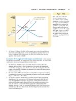
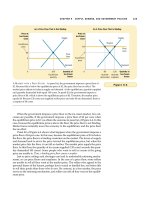
Let’s consider first how the elasticity of supply affects the size of the dead-
weight loss. In the top two panels of Figure 8-5, the demand curve and the size of
the tax are the same. The only difference in these figures is the elasticity of the sup-
ply curve. In panel (a), the supply curve is relatively inelastic: Quantity supplied
responds only slightly to changes in the price. In panel (b), the supply curve is
(a) Inelastic Supply
(b) Elastic Supply
Price
0
Quantity
Price
0
Quantity
Demand
Supply
(c) Inelastic Demand
(d) Elastic Demand
Price
0
Quantity
Price
0
Quantity
Size
of
tax
Size of tax
Demand
Supply
Demand Demand

Supply
Supply
Size
of
tax
Size of tax
When supply is
relatively inelastic,
the deadweight loss
of a tax is small.
When supply is relatively
elastic, the deadweight
loss of a tax is large.
When demand is relatively
elastic, the deadweight
loss of a tax is large.
When demand is
relatively inelastic,
the deadweight loss
of a tax is small.
Figure 8-5
T
AX
D
ISTORTIONS AND
E
LASTICITIES
. In panels (a) and (b), the demand curve and the
size of the tax are the same, but the price elasticity of supply is different. Notice that the
more elastic the supply curve, the larger the deadweight loss of the tax. In panels (c) and

(d), the supply curve and the size of the tax are the same, but the price elasticity of
demand is different. Notice that the more elastic the demand curve, the larger the
deadweight loss of the tax.
168 PART THREE SUPPLY AND DEMAND II: MARKETS AND WELFARE
CASE STUDY
THE DEADWEIGHT LOSS DEBATE
Supply, demand, elasticity, deadweight loss—all this economic theory is enough
to make your head spin. But believe it or not, these ideas go to the heart of a pro-
found political question: How big should the government be? The reason the de-
bate hinges on these concepts is that the larger the deadweight loss of taxation,
the larger the cost of any government program. If taxation entails very large dead-
weight losses, then these losses are a strong argument for a leaner government
that does less and taxes less. By contrast, if taxes impose only small deadweight
losses, then government programs are less costly than they otherwise might be.
So how big are the deadweight losses of taxation? This is a question about
which economists disagree. To see the nature of this disagreement, consider
the most important tax in the U.S. economy—the tax on labor. The Social Se-
curity tax, the Medicare tax, and, to a large extent, the federal income tax are
labor taxes. Many state governments also tax labor earnings. A labor tax places a
wedge between the wage that firms pay and the wage that workers receive. If we
add all forms of labor taxes together, the marginal tax rate on labor income—the
tax on the last dollar of earnings—is almost 50 percent for many workers.
Although the size of the labor tax is easy to determine, the deadweight loss
of this tax is less straightforward. Economists disagree about whether this 50
percent labor tax has a small or a large deadweight loss. This disagreement
arises because they hold different views about the elasticity of labor supply.
Economists who argue that labor taxes are not very distorting believe that
labor supply is fairly inelastic. Most people, they claim, would work full-time
regardless of the wage. If so, the labor supply curve is almost vertical, and a tax
on labor has a small deadweight loss.

Economists who argue that labor taxes are highly distorting believe that la-
bor supply is more elastic. They admit that some groups of workers may supply
their labor inelastically but claim that many other groups respond more to in-
centives. Here are some examples:
◆ Many workers can adjust the number of hours they work—for instance, by
working overtime. The higher the wage, the more hours they choose to work.
relatively elastic: Quantity supplied responds substantially to changes in the price.
Notice that the deadweight loss, the area of the triangle between the supply and
demand curves, is larger when the supply curve is more elastic.
Similarly, the bottom two panels of Figure 8-5 show how the elasticity of de-
mand affects the size of the deadweight loss. Here the supply curve and the size of
the tax are held constant. In panel (c) the demand curve is relatively inelastic, and
the deadweight loss is small. In panel (d) the demand curve is more elastic, and the
deadweight loss from the tax is larger.
The lesson from this figure is easy to explain. A tax has a deadweight loss be-
cause it induces buyers and sellers to change their behavior. The tax raises the price
paid by buyers, so they consume less. At the same time, the tax lowers the price re-
ceived by sellers, so they produce less. Because of these changes in behavior, the
size of the market shrinks below the optimum. The elasticities of supply and de-
mand measure how much sellers and buyers respond to the changes in the price
and, therefore, determine how much the tax distorts the market outcome. Hence,
the greater the elasticities of supply and demand, the greater the deadweight loss of a tax.
CHAPTER 8 APPLICATION: THE COSTS OF TAXATION 169
◆ Some families have second earners—often married women with children—
with some discretion over whether to do unpaid work at home or paid
work in the marketplace. When deciding whether to take a job, these sec-
ond earners compare the benefits of being at home (including savings on
the cost of child care) with the wages they could earn.
◆ Many of the elderly can choose when to retire, and their decisions are partly
based on the wage. Once they are retired, the wage determines their incen-

tive to work part-time.
◆ Some people consider engaging in illegal economic activity, such as the drug
trade, or working at jobs that pay “under the table” to evade taxes. Econo-
mists call this the underground economy. In deciding whether to work in the un-
derground economy or at a legitimate job, these potential criminals compare
what they can earn by breaking the law with the wage they can earn legally.
In each of these cases, the quantity of labor supplied responds to the wage (the
price of labor). Thus, the decisions of these workers are distorted when their la-
bor earnings are taxed. Labor taxes encourage workers to work fewer hours,
second earners to stay at home, the elderly to retire early, and the unscrupulous
to enter the underground economy.
These two views of labor taxation persist to this day. Indeed, whenever you
see two political candidates debating whether the government should provide
more services or reduce the tax burden, keep in mind that part of the disagree-
ment may rest on different views about the elasticity of labor supply and the
deadweight loss of taxation.
“L
ET ME TELL YOU WHAT
I
THINK ABOUT THE ELASTICITY OF LABORSUPPLY
.”
QUICK QUIZ: The demand for beer is more elastic than the demand for
milk. Would a tax on beer or a tax on milk have larger deadweight loss? Why?
170 PART THREE SUPPLY AND DEMAND II: MARKETS AND WELFARE
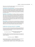
Is there an ideal tax? Henr y
George, the nineteenth-century
American economist and so-
cial philosopher, thought so. In
his 1879 book Progress and
Poverty, George argued that

the government should raise
all its revenue from a tax on
land. This “single tax” was, he
claimed, both equitable and ef-
ficient. George’s ideas won him
a large political following, and
in 1886 he lost a close race for
mayor of New York City (although he finished well ahead of
Republican candidate Theodore Roosevelt).
George’s proposal to tax land was motivated largely
by a concern over the distribution of economic well-being.
He deplored the “shocking contrast between monstrous
wealth and debasing want” and thought landowners bene-
fited more than they should from the rapid growth in the
overall economy.
George’s arguments for the land tax can be understood
using the tools of modern economics. Consider first supply
and demand in the market for renting land. As immigration
causes the population to rise and technological progress
causes incomes to grow, the demand for land rises over
time. Yet because the amount of land is fixed, the supply is
perfectly inelastic. Rapid increases in demand together with
inelastic supply lead to large increases in the equilibrium
rents on land, so that economic growth makes rich landown-
ers even richer.
Now consider the incidence of a tax on land. As we first
saw in Chapter 6, the burden of a tax falls more heavily on
the side of the market that is less elastic. A tax on land takes
this principle to an extreme. Because the elasticity of supply
is zero, the landowners bear the entire burden of the tax.

Consider next the
question of efficiency. As
we just discussed, the
deadweight loss of a tax
depends on the elastici-
ties of supply and de-
mand. Again, a tax on land
is an extreme case. Be-
cause supply is per fectly
inelastic, a tax on land
does not alter the market
allocation. There is no
deadweight loss, and the
government’s tax revenue
exactly equals the loss of
the landowners.
Although taxing land
may look attractive in the-
ory, it is not as straightforward in practice as it may appear.
For a tax on land not to distort economic incentives, it must
be a tax on raw land. Yet the value of land often comes from
improvements, such as clearing trees, providing sewers,
and building roads. Unlike the supply of raw land, the supply
of improvements has an elasticity greater than zero. If a
land tax were imposed on improvements, it would distort in-
centives. Landowners would respond by devoting fewer re-
sources to improving their land.
Today, few economists support George’s proposal for a
single tax on land. Not only is taxing improvements a poten-
tial problem, but the tax would not raise enough revenue to

pay for the much larger government we have today. Yet many
of George’s arguments remain valid. Here is the assess-
ment of the eminent economist Milton Friedman a century
after George’s book: “In my opinion, the least bad tax is the
property tax on the unimproved value of land, the Henry
George argument of many, many years ago.”
H
ENRY
G
EORGE
FYI
Henry George
and the
Land Tax
DEADWEIGHT LOSS AND
TAX REVENUE AS TAXES VARY
Taxes rarely stay the same for long periods of time. Policymakers in local, state,
and federal governments are always considering raising one tax or lowering
another. Here we consider what happens to the deadweight loss and tax revenue
when the size of a tax changes.
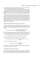
Figure 8-6 shows the effects of a small, medium, and large tax, holding con-
stant the market’s supply and demand curves. The deadweight loss—the reduc-
tion in total surplus that results when the tax reduces the size of a market below
CHAPTER 8 APPLICATION: THE COSTS OF TAXATION 171
the optimum—equals the area of the triangle between the supply and demand
curves. For the small tax in panel (a), the area of the deadweight loss triangle is
quite small. But as the size of a tax rises in panels (b) and (c), the deadweight loss
grows larger and larger.
Indeed, the deadweight loss of a tax rises even more rapidly than the size of
the tax. The reason is that the deadweight loss is an area of a triangle, and an area

Demand
Supply
P
B
Quantity
Q
2
0
Price
Q
1
Demand
Supply
(a) Small Tax
Deadweight
loss
Tax revenue
Tax revenue
P
S
P
B
Quantity
Q
2
0
Price
Q
1
(b) Medium Tax

Deadweight
loss
P
S
Figure 8-6
D
EADWEIGHT
L
OSS AND
T
AX
R
EVENUE FROM
T
HREE
T
AXES OF
D
IFFERENT
S
IZE
. The
deadweight loss is the reduction in total surplus due to the tax. Tax revenue is the amount
of the tax times the amount of the good sold. In panel (a), a small tax has a small
deadweight loss and raises a small amount of revenue. In panel (b), a somewhat larger tax
has a larger deadweight loss and raises a larger amount of revenue. In panel (c), a very
large tax has a very large deadweight loss, but because it has reduced the size of the
market so much, the tax raises only a small amount of revenue.
Tax revenue
P

B
Quantity
Q
2
0
Price
Q
1
Demand
Supply
(c) Large Tax
Deadweight
loss
P
S