Tài liệu Ten Principles of Economics - Part 69 pdf

CHAPTER 31 AGGREGATE DEMAND AND AGGREGATE SUPPLY 705
FACT 3: AS OUTPUT FALLS, UNEMPLOYMENT RISES
Changes in the economy’s output of goods and services are strongly correlated
with changes in the economy’s utilization of its labor force. In other words, when
real GDP declines, the rate of unemployment rises. This fact is hardly surprising:
When firms choose to produce a smaller quantity of goods and services, they lay
off workers, expanding the pool of unemployed.
Panel (c) of Figure 31-1 shows the unemployment rate in the U.S. economy
since 1965. Once again, recessions are shown as the shaded areas in the figure. The
figure shows clearly the impact of recessions on unemployment. In each of the re-
cessions, the unemployment rate rises substantially. When the recession ends and
real GDP starts to expand, the unemployment rate gradually declines. The unem-
ployment rate never approaches zero; instead, it fluctuates around its natural rate
of about 5 percent.
QUICK QUIZ: List and discuss three key facts about economic fluctuations.
EXPLAINING SHORT-RUN
ECONOMIC FLUCTUATIONS
Describing the regular patterns that economies experience as they fluctuate over
time is easy. Explaining what causes these fluctuations is more difficult. Indeed,
compared to the topics we have studied in previous chapters, the theory of eco-
nomic fluctuations remains controversial. In this and the next two chapters, we de-
velop the model that most economists use to explain short-run fluctuations in
economic activity.
HOW THE SHORT RUN DIFFERS FROM THE LONG RUN
In previous chapters we developed theories to explain what determines most im-
portant macroeconomic variables in the long run. Chapter 24 explained the level
and growth of productivity and real GDP. Chapter 25 explained how the real in-
terest rate adjusts to balance saving and investment. Chapter 26 explained why
there is always some unemployment in the economy. Chapters 27 and 28 ex-
plained the monetary system and how changes in the money supply affect the
price level, the inflation rate, and the nominal interest rate. Chapters 29 and 30 ex-

tended this analysis to open economies in order to explain the trade balance and
the exchange rate.
All of this previous analysis was based on two related ideas—the classical di-
chotomy and monetary neutrality. Recall that the classical dichotomy is the sepa-
ration of variables into real variables (those that measure quantities or relative
prices) and nominal variables (those measured in terms of money). According to
classical macroeconomic theory, changes in the money supply affect nominal vari-
ables but not real variables. As a result of this monetary neutrality, Chapters 24, 25,
706 PART TWELVE SHORT-RUN ECONOMIC FLUCTUATIONS
and 26 were able to examine the determinants of real variables (real GDP, the real
interest rate, and unemployment) without introducing nominal variables (the
money supply and the price level).
Do these assumptions of classical macroeconomic theory apply to the world in
which we live? The answer to this question is of central importance to under-
standing how the economy works: Most economists believe that classical theory de-
scribes the world in the long run but not in the short run. Beyond a period of several
years, changes in the money supply affect prices and other nominal variables but
do not affect real GDP, unemployment, or other real variables. When studying
year-to-year changes in the economy, however, the assumption of monetary neu-
trality is no longer appropriate. Most economists believe that, in the short run, real
and nominal variables are highly intertwined. In particular, changes in the money
supply can temporarily push output away from its long-run trend.
To understand the economy in the short run, therefore, we need a new model.
To build this new model, we rely on many of the tools we have developed in pre-
vious chapters, but we have to abandon the classical dichotomy and the neutrality
of money.
THE BASIC MODEL OF ECONOMIC FLUCTUATIONS
Our model of short-run economic fluctuations focuses on the behavior of two vari-
ables. The first variable is the economy’s output of goods and services, as mea-
sured by real GDP. The second variable is the overall price level, as measured by

the CPI or the GDP deflator. Notice that output is a real variable, whereas the price
level is a nominal variable. Hence, by focusing on the relationship between these
two variables, we are highlighting the breakdown of the classical dichotomy.
We analyze fluctuations in the economy as a whole with the model of aggre-
gate demand and aggregate supply, which is illustrated in Figure 31-2. On the ver-
tical axis is the overall price level in the economy. On the horizontal axis is the
overall quantity of goods and services. The aggregate-demand curve shows the
quantity of goods and services that households, firms, and the government want
to buy at each price level. The aggregate-supply curve shows the quantity of
goods and services that firms produce and sell at each price level. According to
this model, the price level and the quantity of output adjust to bring aggregate de-
mand and aggregate supply into balance.
It may be tempting to view the model of aggregate demand and aggregate
supply as nothing more than a large version of the model of market demand and
market supply, which we introduced in Chapter 4. Yet in fact this model is quite
different. When we consider demand and supply in a particular market—ice
cream, for instance—the behavior of buyers and sellers depends on the ability of
resources to move from one market to another. When the price of ice cream rises,
the quantity demanded falls because buyers will use their incomes to buy prod-
ucts other than ice cream. Similarly, a higher price of ice cream raises the quantity
supplied because firms that produce ice cream can increase production by hiring
workers away from other parts of the economy. This microeconomic substitution
from one market to another is impossible when we are analyzing the economy as
a whole. After all, the quantity that our model is trying to explain—real GDP—
measures the total quantity produced in all of the economy’s markets. To under-
stand why the aggregate-demand curve is downward sloping and why the
model of aggregate
demand and
aggregate supply
the model that most economists

use to explain short-run
fluctuations in economic activity
around its long-run trend
aggregate-demand curve
a curve that shows the quantity of
goods and services that households,
firms, and the government want to
buy at each price level
aggregate-supply curve
a curve that shows the quantity of
goods and services that firms choose
to produce and sell at each price level
CHAPTER 31 AGGREGATE DEMAND AND AGGREGATE SUPPLY 707
aggregate-supply curve is upward sloping, we need a macroeconomic theory.
Developing such a theory is our next task.
QUICK QUIZ: How does the economy’s behavior in the short run differ
from its behavior in the long run? ◆ Draw the model of aggregate demand
and aggregate supply. What variables are on the two axes?
THE AGGREGATE-DEMAND CURVE
The aggregate-demand curve tells us the quantity of all goods and services de-
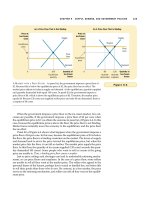
manded in the economy at any given price level. As Figure 31-3 illustrates, the
aggregate-demand curve is downward sloping. This means that, other things
equal, a fall in the economy’s overall level of prices (from, say, P
1
to P
2
) tends to
raise the quantity of goods and services demanded (from Y
1
to Y

2
).
WHY THE AGGREGATE-DEMAND CURVE
SLOPES DOWNWARD
Why does a fall in the price level raise the quantity of goods and services de-
manded? To answer this question, it is useful to recall that GDP (which we denote
as Y) is the sum of consumption (C), investment (I), government purchases (G),
and net exports (NX):
Equilibrium
output
Quantity of
Output
Price
Level
0
Equilibrium
price level
Aggregate
supply
Aggregate
demand
Figure 31-2
A
GGREGATE
D
EMAND
AND
A
GGREGATE
S

UPPLY
.
Economists use the model of
aggregate demand and aggregate
supply to analyze economic
fluctuations. On the vertical
axis is the overall level of prices.
On the horizontal axis is the
economy’s total output of
goods and services. Output
and the price level adjust
to the point at which
the aggregate-supply
and aggregate-demand
curves intersect.
708 PART TWELVE SHORT-RUN ECONOMIC FLUCTUATIONS
Y ϭ C ϩ I ϩ G ϩ NX.
Each of these four components contributes to the aggregate demand for goods and
services. For now, we assume that government spending is fixed by policy. The
other three components of spending—consumption, investment, and net ex-
ports—depend on economic conditions and, in particular, on the price level. To un-
derstand the downward slope of the aggregate-demand curve, therefore, we must
examine how the price level affects the quantity of goods and services demanded
for consumption, investment, and net exports.
The Price Level and Consumption: The Wealth Effect
Con-
sider the money that you hold in your wallet and your bank account. The nominal
value of this money is fixed, but its real value is not. When prices fall, these dollars
are more valuable because then they can be used to buy more goods and services.
Thus, a decrease in the price level makes consumers feel more wealthy, which in turn en-

courages them to spend more. The increase in consumer spending means a larger quantity
of goods and services demanded.
The Price Level and Investment: The Interest-Rate Effect
As we discussed in Chapter 28, the price level is one determinant of the quantity
of money demanded. The lower the price level, the less money households need to
hold to buy the goods and services they want. When the price level falls, therefore,
households try to reduce their holdings of money by lending some of it out. For in-
stance, a household might use its excess money to buy interest-bearing bonds. Or
it might deposit its excess money in an interest-bearing savings account, and the
bank would use these funds to make more loans. In either case, as households try
to convert some of their money into interest-bearing assets, they drive down
Quantity of
Output
Price
Level
0
Aggregate
demand
P
1
Y
1
Y
2
P
2
1. A decrease
in the price
level . . .
2. . . . increases the quantity of

goods and services demanded.
Figure 31-3
T
HE
A
GGREGATE
-D
EMAND
C
URVE
. A fall in the price level
from P
1
to P
2
increases the
quantity of goods and services
demanded from Y
1
to Y
2
. There
are three reasons for this negative
relationship. As the price level
falls, real wealth rises, interest
rates fall, and the exchange rate
depreciates. These effects
stimulate spending on
consumption, investment, and
net exports. Increased spending

on these components of output
means a larger quantity of goods
and services demanded.
CHAPTER 31 AGGREGATE DEMAND AND AGGREGATE SUPPLY 709
interest rates. Lower interest rates, in turn, encourage borrowing by firms that
want to invest in new plants and equipment and by households who want to in-
vest in new housing. Thus, a lower price level reduces the interest rate, encourages
greater spending on investment goods, and thereby increases the quantity of goods and
services demanded.
The Price Level and Net Exports: The Exchange-Rate Ef-
fect
As we have just discussed, a lower price level in the United States lowers
the U.S. interest rate. In response, some U.S. investors will seek higher returns by
investing abroad. For instance, as the interest rate on U.S. government bonds falls,
a mutual fund might sell U.S. government bonds in order to buy German govern-
ment bonds. As the mutual fund tries to move assets overseas, it increases the sup-
ply of dollars in the market for foreign-currency exchange. The increased supply
of dollars causes the dollar to depreciate relative to other currencies. Because each
dollar buys fewer units of foreign currencies, foreign goods become more expen-
sive relative to domestic goods. This change in the real exchange rate (the relative
price of domestic and foreign goods) increases U.S. exports of goods and services
and decreases U.S. imports of goods and services. Net exports, which equal ex-
ports minus imports, also increase. Thus, when a fall in the U.S. price level causes U.S.
interest rates to fall, the real exchange rate depreciates, and this depreciation stimulates
U.S. net exports and thereby increases the quantity of goods and services demanded.
Summary
There are, therefore, three distinct but related reasons why a fall in
the price level increases the quantity of goods and services demanded: (1) Con-
sumers feel wealthier, which stimulates the demand for consumption goods. (2)
Interest rates fall, which stimulates the demand for investment goods. (3) The ex-

change rate depreciates, which stimulates the demand for net exports. For all three
reasons, the aggregate-demand curve slopes downward.
It is important to keep in mind that the aggregate-demand curve (like all de-
mand curves) is drawn holding “other things equal.” In particular, our three ex-
planations of the downward-sloping aggregate-demand curve assume that the
money supply is fixed. That is, we have been considering how a change in the
price level affects the demand for goods and services, holding the amount of
money in the economy constant. As we will see, a change in the quantity of money
shifts the aggregate-demand curve. At this point, just keep in mind that the
aggregate-demand curve is drawn for a given quantity of money.
WHY THE AGGREGATE-DEMAND CURVE MIGHT SHIFT
The downward slope of the aggregate-demand curve shows that a fall in the price
level raises the overall quantity of goods and services demanded. Many other fac-
tors, however, affect the quantity of goods and services demanded at a given price
level. When one of these other factors changes, the aggregate-demand curve shifts.
Let’s consider some examples of events that shift aggregate demand. We can
categorize them according to which component of spending is most directly
affected.
Shifts Arising from Consumption
Suppose Americans suddenly be-
come more concerned about saving for retirement and, as a result, reduce their
current consumption. Because the quantity of goods and services demanded at