Tài liệu HPLC for Pharmaceutical Scientists 2007 (Part 2) pptx

2
HPLC THEORY
Yuri Kazakevich
2.1 INTRODUCTION
The process of analyte retention in high-performance liquid chromatography
(HPLC) involves many different aspects of molecular behavior and interac-
tions in condensed media in a dynamic interfacial system. Molecular diffusion
in the eluent flow with complex flow dynamics in a bimodal porous space is
only one of many complex processes responsible for broadening of the chro-
matographic zone. Dynamic transfer of the analyte molecules between mobile
phase and adsorbent surface in the presence of secondary equilibria effects is
also only part of the processes responsible for the analyte retention on the
column. These processes just outline a complex picture that chromatographic
theory should be able to describe.
HPLC theory could be subdivided in two distinct aspects: kinetic and ther-
modynamic. Kinetic aspect of chromatographic zone migration is responsible
for the band broadening, and the thermodynamic aspect is responsible for the
analyte retention in the column. From the analytical point of view, kinetic
factors determine the width of chromatographic peak whereas the thermody-
namic factors determine peak position on the chromatogram. Both aspects are
equally important, and successful separation could be achieved either by opti-
mization of band broadening (efficiency) or by variation of the peak positions
on the chromatogram (selectivity). From the practical point of view, separa-
tion efficiency in HPLC is more related to instrument optimization, column
25
HPLC for Pharmaceutical Scientists, Edited by Yuri Kazakevich and Rosario LoBrutto
Copyright © 2007 by John Wiley & Sons, Inc.
dimensions, and particle geometry—factors that could not have continuous
variation during method development except for the small influence from vari-
ation of the mobile phase flow rate. On the other hand, analyte retention or
selectivity is mainly dependent on the competitive intermolecular interactions

and are influenced by eluent type, composition, temperature, and other vari-
ables which allow functional variation.
2.2 BASIC CHROMATOGRAPHIC DESCRIPTORS
Four major descriptors are commonly used to report characteristics of the
chromatographic column, system, and particular separation:
1. Retention factor (k)
2. Efficiency (N)
3. Selectivity (α)
4. Resolution (R)
Retention factor (k) is the unitless measure of the retention of a particular com-
pound on a particular chromatographic system at given conditions defined as
(2-1)
where V
R
is the analyte retention volume, V
0
is the volume of the liquid phase
in the chromatographic system, t
R
is the analyte retention time, and t
0
is some-
times defined as the retention time of nonretained analyte. Retention factor
is convenient because it is independent on the column dimensions and mobile-
phase flow rate. Note that all other chromatographic conditions significantly
affect retention factor.
Efficiency is the measure of the degree of peak dispersion in a particular
column; as such, it is essentially the characteristic of the column. Efficiency is
expressed in the number of theoretical plates (N) calculated as
(2-2)

where t
R
is the analyte retention time and w is the peak width at the baseline.
Selectivity (α) is the ability of chromatographic system to discriminate two
different analytes. It is defined as the ratio of corresponding retention factors:
(2-3)
α=
k
k
2
1
N
t
w
R
=




16
2
k
VV
V
tt
t
RR
=
−

=
−
0
0
0
0
26 HPLC THEORY
Resolution (R) is a combined measure of the separation of two compounds
which include peak dispersion and selectivity. Resolution is defined as
(2-4)
In the following sections the chromatographic descriptors introduced above
[equations (2-1)–(2-4)] will be discussed in terms of their functional depen-
dencies, specifics, and relationships with different chromatographic and ther-
modynamic parameters.
2.3 EFFICIENCY
The most rigorous discussion of the formation of chromatographic zone and
the mathematical description of zone-broadening is given in reference 1. Here
only practically important and useful equations will be discussed.
If column properties could be considered isotropic, then we would expect
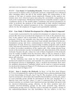
symmetrical peaks of a Gaussian shape (Figure 2-1), and the variance of this
peak is proportional to the diffusion coefficient (D)
(2-5)
At given linear velocity (ν) the component moves through the column with
length (L) during the time (t), or
(2-6)
Lvt=
σ
2
2= Dt
R

tt
ww
=
−
+
2
21
21
EFFICIENCY 27
Figure 2-1. Gaussian band broadening
.
Substituting t from equation (2-6) in equation (2-5), we get
(2-7)
Expression 2D/ν has units of length and is essentially the measure of band
spreading at a given velocity on the distance L of the column. This parameter
has essentially the sense of the height equivalent to the theoretical plate and
could be denoted as H, so we get
(2-8)
Several different processes lead to the band-spreading phenomena in the
column which include: multipath effect; molecular diffusion; displacement in
the porous beds; secondary equilibria; and others. Each of these processes
introduces its own degree of variance toward the overall band-spreading
process. Usually these processes are assumed to be independent; and based on
the fundamental statistical law, overall band-spreading (variance) is equal to
the sum of the variances for each independent process:
(2-9)
In the further discussion we assume the total variance in all cases.
In the form of equation (2-8) the definition of H is exactly identical to the
plate height as it evolved from the distillation theory and was brought to chro-
matography by Martin and Synge [2]. If H is the theoretical plate height, we

can determine the total number of the theoretical plates in the column as
(2-10)
In linear chromatography, each analyte travels through the column with con-
stant velocity (u
c
). Using this velocity, we can express the analyte retention
time as
(2-11)
Similarly, the time necessary to move analyte zone in the column on the dis-
tance of one σ (Figure 2-1) can be defined as t
(2-12)
τ
σ
=
u
c
t
L
u
R
c
=
N
L
H
N
L
=⇒=





σ
2
σσ
tot
22
=
∑
i
H
L
=
σ
2
σ
2
2
=




D
v
L
28 HPLC THEORY
Substituting both equations (2-11) and (2-12) into (2-10), we get
(2-13)
Parameter t in equation (2-13) is the standard deviation and expressed in

the same units as retention time. Since we considered symmetrical band-
broadening of a Gaussian shape, we can use Gaussian function to relate its
standard deviation to more easily measurable quantities. The most commonly
used points are the so-called peak width at the baseline, which is actually the
distance between the points of intersections of the tangents to the peaks inflec-
tion points with the baseline (shown in Figure 2-1). This distance is equal to
four standard deviations, and the final equation for efficiency will be
(2-14)
Another convenient determination for N is by using the peak width at the half-
height. From the same Gaussian function the peak width on the half-height is
2.355 times longer than the standard deviation of the same peak, and the
resulting formula for the number of the theoretical plates will be
(2-15)
Efficiency is mainly a column-specific parameter. In a gas chromatography
column, efficiency is highly dependent on the flow rate. In HPLC, because of
much higher viscosity, the applicable flow rate region is not so broad; within
this region, variations of the flow rate do not affect column efficiency signifi-
cantly.
On the other hand, geometry of the packing material and uniformity and
density of the column packing are the main factors defining the efficiency of
particular column.There is no clear fundamental relationship between the par-
ticle diameter and the expected column efficiency, but phenomenologically an
increase of the efficiency can be expected with the decrease of the particle
diameter, since the difference between the average size of the pores in the par-
ticles of the packing material and the effective size of interparticle pores
decreases, which leads to the more uniform flow inside and around the parti-
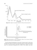
cles. From Figure 2-2 it is obvious that the smaller the particles, the lower the
theoretical plate height and the higher the efficiency. The general form of
the shown dependence is known as Van Deemter function (2-16), which has
the following mathematical form:

(2-16)
HA
B
v
Cv=++
N
t
w
R
h
=






5 545
1
2
2
.
N
t
w
r
b
=





16
2
N
t
R
=




τ
2
EFFICIENCY 29
where ν is the linear flow velocity, and A, B, and C are constants for given
column and mobile phase.
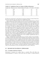
Three terms of the above equation essentially represent three different
processes that contribute to the overall chromatographic band-broadening.
A—represents multipath effect or eddy diffusion
B—represents molecular diffusion
C—represents mass transfer
The multipath effect is a flow-independent term, which defines the ability of
different molecules to travel through the porous media with paths of differ-
ent length.
The molecular diffusion term is inversely proportional to the flow rate,
which means that the slower the flow rate, the longer component stays in the
column and the molecular diffusion process has more time to broaden the
peak.
The mass-transfer term is proportional to the flow rate, which means that

the faster the flow, the greater the band-broadening. Superposition of all three
processes is shown schematically in Figure 2-3.
As it could be seen from the comparison of Figure 2-2 and Figure 2-3, all
dependencies of the column efficiency on the flow rate follow the theoretical
Van Deemter curve.In theory there is an optimum flow rate that allows obtain-
ing the highest efficiency (the lower theoretical plate height).
30 HPLC THEORY
Figure 2-2. The experimental dependence of the theoretical plate height on the flow
velocity for columns packed with same type of particles of different average diameter.
As follows from Figure 2-2, the lower the particle diameter, the wider the
range of the flow rates where the highest column efficiency is achieved. For
columns packed with smaller particles, efficiency is not as adversely affected
at faster flow rates, because the mass-transfer term is lower for these columns.
Essentially, this means that retention equilibrium is achieved much faster in
these columns.
Faster flow rates mean higher flow resistance and higher backpressure. It is
a modern trend to work with the smaller particles at high linear velocity.
However, the overall efficiency of the columns packed with smaller particles
(<2µm) is not much higher compared to conventional columns with 3- to 5-µ
particles. The comparison of a conventional 15-cm column with 4.6-mm inter-
nal diameter packed with 5-µm particles to a column of 15-cm length and
2-mm I.D. packed with 1.7-µm particles shows that the average efficiency of
the first column is between 12,000 and 15,000 theoretical plates, and for the
second column the efficiency is not much higher: It is on the level of 15,000 to
18,000 theoretical plates.This small increase of the efficiency may only slightly
improve the separation; however, the comparison of the run times at the same
volumetric flow rates on both columns shows that the separation on the second
column can be achieved five times faster.
Of course, the ability to increase u depends on the pressure capabilities of
the instrument, since pressure is directly proportional to velocity:

(2-17)
∆P
uL
d
p
=
hf
2
EFFICIENCY 31
Figure 2-3. Schematic of the Van Deemter function and its components.
where ∆P is the pressure drop across the column, h is viscosity, and f is the
flow resistance factor [3]. Therefore, the fastest possible separation requires
that the maximum pressure allowed by the instrument be used, assuming that
the resolution requirement can still be met. This also means that the speed of
analysis is limited by that maximum pressure. As a result, one wants to make
the most of the pressure available by reducing the pressure drop across the
column as much as possible. This can be achieved by working at higher tem-
peratures,using MeCN/water mobile phases instead of methanol/water mobile
phases on the same length of column or by using shorter columns.
To limit analysis time, the shortest column length possible should be used.
Shorter columns have lower pressure requirements, allowing to gain an advan-
tage in speed. It must be kept in mind, however, that N will decrease as u
increases (for particles ≥3µm), meaning that at faster velocities longer
columns are necessary to give the required theoretical plates, thus generating
greater operating pressures.
2.4 RESOLUTION
In the introduction section we define the term resolution as the ability of the
column to resolve two analyte in two separate peaks (or chromatographic
zones). In more general form than it was given before, the resolution can be
defined as the half of the distance between the centers of gravity of two chro-

matographic zones related to the sum of their standard deviations:
(2-18)
In case of symmetrical peaks, centers of peak gravity could be substituted with
the peak maxima; and using the relationship of the peak width with its stan-
dard deviation (shown in Figure 2-1), a common expression for the resolution
could be obtained:
(2-19)
The peak width in equation (2-19) could be substituted using expression
(2-14), and the resulting equation is
(2-20)
Expression (2-20) demonstrates that resolution is proportional to the square
root of the efficiency.
R
tt
tt
N
RR
RR
=
−
+
⋅
21
21
2
R
tt
ww
RR
=

−
+
()
21
21
1
2
R
XX
=
−
+
()
21
12
2 σσ
32 HPLC THEORY
From the practical point of view, in case of the lack of resolution for some
specific separation there are generally two ways to improve it: Increase the
efficiency, or increase the selectivity. The efficiency is proportional to the
column length: The longer the column, the higher the efficiency, but equation
(2-20) shows that the increase of the efficiency increases the resolution only
as a square root function (as illustrated in Figure 2-4). At the same time, the
increase of the column length leads to the increase of the flow resistance and
backpressure, which limits the ability to further increase the column length.
If we assume that the peak widths of two adjacent peaks are approximately
equal, we can rewrite expression (2-18) in the form
(2-21)
For symmetrical chromatographic bands, this is the ratio of the distance
between peaks maxima to the peak width.The distance between peak maxima

is proportional to the distance of the chromatographic zone migration, and the
peak width is proportional to the square root of this distance. Figure 2-4 illus-
trates this relationship.
At low selectivity to achieve the same resolution, one has to use a longer
column to increase efficiency and consequently operate under higher-pressure
conditions. The relationship between the column length, mobile-phase viscos-
ity, and the backpressure is given by equation (2-17), which is the variation of
the Kozeny–Carman equation. Expression (2-17) predicts a linear increase of
the backpressure with the increase of the flow rate, column length, and mobile
phase viscosity.The decrease of the particle diameter, on the other hand, leads
to the quadratic increase of the column backpressure.
Achievement of good resolution between analytes in complex chro-
matogram is the main goal in HPLC method development. Optimal resolu-
tion could be achieved by optimization of system efficiency, or selectivity (or
R
XX
=
−
21
4σ
RESOLUTION 33
Figure 2-4. Relationship between resolution, selectivity, and column length.
both). Relationships of the retention, selectivity, and efficiency with the reso-
lution has been for long a subject of extensive theoretical studies [4–6], with
the goal to express resolution as a function of k, a, and N.
Unfortunately, the direct algebraic transformation of expression (2-19) into
some form of functional dependence of R on k, α, and N is impossible. Knox
and Thijssen were the first to independently propose the transformation based
on the assumption of equal peak width (w
2

= w
1
) and consideration of the
retention of the first peak of the pair (k
1
). The resulting expression is
(2-22)
For closely eluted peaks and relatively high efficiency of the system, these
assumptions do not lead to the significant deviations of equation (2-22) from
true resolution given by equation (2-19).
Purnell [7] suggested to center attention on the second peak of the pair,
thus using the peak width of the second component as a base width (meaning
that the width of the first peak is equal to the width of the second peak). This
assumption leads to the following equation:
(2-23)
Both equations do not give a real resolution value; also, the greater the dis-
tance between peaks, the higher the error.
Said [6] suggests the use of average values instead of selection of the first
or second primary peaks, which leads to the following expression for resolu-
tion:
(2-24)
All these expressions give approximate values of resolution; also, the smaller
the distance between target peaks in the chromatogram, the closer the values
to the true resolution. Detailed analysis of available master resolution equa-
tions is given in the B. Karger article [4].
2.5 HPLC RETENTION
In Section 2.1 the main chromatographic descriptors generally used in routine
HPLC work were briefly discussed. Retention factor and selectivity are the
parameters related to the analyte interaction with the stationary phase and
reflect the thermodynamic properties of chromatographic system. Retention

factor is calculated using expression (2-1) from the analyte retention time or
retention volume and the total volume of the liquid in the column. Retention
R
k
k
N
=
−
+




+




a
a
1
1
1
2
R
k
k
N
=
+





−




2
2
1
1
4
a
a
R
k
k
N
=
+




−
()
1
1

1
1
4
a
34 HPLC THEORY
time (t
R
) is essentially equivalent to the retention volume (t
R
× flow rate),
provided that the mobile-phase flow rate was constant throughout the whole
separation process.
Part of the total retention volume of the analyte is the void volume. Even
if the analyte molecules do not interact with the column packing material, the
analyte needs some time to pass through the column.This time is usually called
hold-up time, dead time, or void time. The corresponding volume is either the
void volume, the volume of the liquid phase in the column, or the dead volume.
Analyte retention volume that exceeds the column void volume is essentially
the volume of the mobile phase which had passed through the column while
analyte molecules were retained by the packing material.
To derive the relationship of the analyte retention with the thermodynamic
properties of chromatographic system, the mechanism of the analyte behav-
ior in the column should be determined. The mechanism and the theoretical
description of the analyte retention in HPLC has been the subject of many
publications, and different research groups are still in disagreement on what
is the most realistic retention mechanism and what is the best theory to
describe the analyte retention and if possible predict its behavior [8, 9].
2.6 RETENTION MECHANISM
Almost 30 years ago, Colin and Guiochon mentioned in an excellent review
[10] that there are essentially three possible ways to model separation mech-

anism. The first one is analyte partitioning between mobile and stationary
phases, the second one is the adsorption of the analyte on the surface of non-
polar adsorbent, and the third one has been suggested by Knox and Pryde [11],
where they assume the preferential adsorption of the organic mobile-phase
modifier on the adsorbent surface followed by the analyte partitioning into
this adsorbed layer.
Partitioning is the first and probably the simplest model of the retention
mechanism. It assumes the existence of two different phases (mobile and sta-
tionary) and instant equilibrium of the analyte partitioning between these
phases. Simple phenomenological interpretation of the dynamic partitioning
process was also introduced at about the same time. Probably, the most con-
sistent and understandable description of this theory is given by C. Cramers,
A. Keulemans, and H. McNair in 1961 in their chapter “Techniques of Gas
Chromatography” [12]. The analyte partition coefficient is defined as
(2-25)
and the analyte retention factor is defined as the ratio of the total amount of
analyte in the stationary phase to the total amount of analyte in the mobile
phase
K
c
c
S
M
=
RETENTION MECHANISM 35
(2-26)
The fraction of the analyte in the mobile phase could be written in the form
(2-27)
and is regarded as the retardation factor. It is then assumed that R
f

could be
considered as the fraction of time which a component spends in the mobile
phase and by multiplying mobile-phase velocity on R
f
the average component
velocity in the column is obtained.
(2-28)
where u it the mobile-phase linear velocity and u
c
is the velocity of the analyte.
The retention time is the ratio of the column length and analyte velocity, thus
(2-29)
Converting expression (2-29) into retention volumes using V
R
= Ft
R
and V
m
= F
t0
,
where F is the mobile-phase flow rate, and combining with (2-26) we get
(2-30)
Later these mnemonic derivations appear in all textbooks dealing with gas and
liquid chromatography. Equation (2-30) describes the retention of the analyte,
which undergoes only one process of ideal partitioning between well-defined
mobile and stationary phases.
In gas chromatography the analyte partitioning between mobile gas phase
and stationary liquid phase is a real retention mechanism; also, phase para-
meters, such as volume, thickness, internal diameter, and so on, are well known

and easily determined. In liquid chromatography, however, the correct defin-
ition of the mobile-phase volume has been a subject of continuous debate in
the last 30 years [13–16]. The assumption that the retardation factor, R
f
, which
is a quantitative ratio, could be considered as the fraction of time that com-
ponents spend in the mobile phase is not obvious either.
The phenomenological description of the retention mechanism discussed
above is only applicable for the system with single partitioning process and
well-defined stationary and mobile phases. A more general method for the
derivation of retention function is based on the solution of column mass
balance [17].
VVVK
Rms
=+
t
L
u
kt k
R
=+
()
=+
()
11
0
uu
k
c
=

+
1
1
R
q
qq k
f
M
SM
=
+
=
+
1
1
k
q
q
Vc
Vc
V
V
K
S
M
SS
MM
S
M
==

=
36 HPLC THEORY
2.7 GENERAL COLUMN MASS BALANCE
Analyte transport through the HPLC column is considered to be one-
dimensional along the axis x of the column, as shown in Figure 2-5.The analyte
in the column slice dx is considered to be in instantaneous thermodynamic
equilibrium. Various processes in which analyte could be involved (e.g., ion-
ization, solvation, tatutomerism) are also considered to be at the equilibrium.
To simplify the discussion and allow for the analytical solution of mass balance
equation, the absence of the axial analyte dispersion is assumed.
The following assumptions on the behavior of the chromatographic systems
are made:
1. Molar volumes of the analyte and mobile-phase components are con-
stant, and compressibility of the liquid phase is negligible.
2. Adsorbent is rigid material impermeable for the analyte and mobile-
phase components.
3. Adsorbent is characterized by its specific surface area and pore volume,
which are evenly distributed axially and radially in the column. (This
assumption is equivalent to the assumption of column homogeneity.)
4. Thermal effects are negligible.
5. System is at instant thermodynamic equilibrium.
The column void volume, V
0
, is defined as the total volume of the liquid phase
in the column and could be measured independently [18]. Total adsorbent
surface area in the column, S, is determined as the product of the adsorbent
mass and specific surface area.
Considering the classical picture of the column slice (Figure 2-5) with the
mobile-phase flow rate F and length L packed with small porous particles, the
analyte injected at x = 0 will be carried through the column with the mobile

phase and its concentration in any part of the column is a function of the dis-
tance from the inlet x and the time t. The amount of the analyte entering the
GENERAL COLUMN MASS BALANCE 37
Figure 2-5. Illustration of the column slice for construction of mass balance. Mobile-
phase flow F in mL/min; analyte concentration c in mol/L; n is the analyte accumula-
tion in the slice dx in mol; v is the mobile-phase volume in the slice dx expressed as
V
0
/L, where L is the column length; s is the adsorbent surface area in the slice dx,
expressed as S/L, where S is the total adsorbent area in the column.
cross-sectional zone dx during the time dt is equal to Fcdt. During the same
time dt the amount of analyte leaving the zone dx could be expressed as F(c
+ dc)dt. The difference in the analyte amount entering zone dx and exiting it
at the same time dt will be Fdcdt. Note that dc could be positive or negative.
The analyte accumulation in the zone dx could be expressed in the form of
the gradient of the concentration along the column axis (x)
(2-31)
Equation (2-31) represents the analyte amount accumulated in the zone dx
during the time dt. This amount undergoes some distribution processes in the
selected zone. These processes are the actual reason for the analyte accumu-
lation.The analyte distribution function in the selected zone is the second half
of the mass balance equation; the amount of analyte accumulated in zone dx
should be equal to the amount distributed inside this zone. In general form, it
could be written as
(2-32)
where the analyte concentration is a function of both the distance and the time
and y(c) is a distribution function that has units of the analyte amount per
unit length of the column.This distribution function is the key for the solution
of equation (2-32), and the definition of this function essentially determines
how chromatographic retention will be described.

Equation (2-32) is simplified to
(2-33)
This equation states that the formation of the analyte concentrational gradi-
ent in a fixed moment of time in any place of the column should be equal to
the time-dependent variation of the analyte amount.
The general solution of equation (2-33) could be obtained using two clas-
sical relationships for partial derivatives [for simple forms of the distribution
function y(c)]
(2-34)
(2-35)
Substitution of equation (2-34) into equation (2-33) gives
(2-36)
−




=
()








F
c
x

dc
dc
c
t
t
x
x
∂
∂
∂
∂
y
∂
∂
∂
∂
∂
∂
c
t
c
x
x
t
xtc




=





⋅




∂
∂
∂
∂
∂
∂
y
t
y
c
c
t
xxx




=





⋅




−




=
()




F
c
x
c
t
tx
∂
∂
∂
∂
y
−





=
()




F
c
x
dxdt
c
t
dxdt
tx
∂
∂
∂
∂
y
Fdcdc F
c
x
dxdt
t
=−





∂
∂
38 HPLC THEORY
The partial derivative of the distribution function by the concentration is actu-
ally a full derivative since it is independent on the time and position of the
analyte in the column given that the chromatographic system is at the equi-
librium. Applying relationship (2-35), we get
(2-37)
The term (∂x/∂t)
c
is linear velocity of the analyte at concentration c and can
be denoted as u
c
.
The final form of the simplified mass balance solution is
(2-38)
Since V
R
= FL/u
c
, where L is the column length, equation (2-38) could be
written in its final form
(2-39)
The retention volume is essentially proportional to the derivative of the
analyte distribution function defined per unit of the column length.
Further development of the mathematical description of the chromato-
graphic process requires the definition of the analyte distribution function
y(c), or essentially the introduction of the retention model (or mechanism).

2.8 PARTITIONING MODEL
As a first example of an applicable model traditional partitioning mechanism
will be considered. In this mechanism the analyte is distributed between the
mobile and stationary phases, and phenomenological description of this
process is given in Section 2.1. The V
m
and V
s
are the volume of the mobile
and the volume of the stationary phases in the column, respectively. Instant
equilibrium of the analyte distribution between mobile and stationary phases
is assumed.
The total amount of the analyte in the column cross section dx is distrib-
uted between the mobile and stationary phases and could be written in the
following form:
(2-40)
y cvcvc
ss mm
()
=+
Vc L
dc
dc
R
()
=⋅
()
y
u
F

dc
dc
c
=
()
y
F
c
x
dc
dc
c
x
x
t
F
dc
dc
x
t
ttc c
∂
∂
∂
∂
∂
∂
∂
∂





=
()








⇒=
()




yy
PARTITIONING MODEL 39
where ν
s
and c
s
are the volumes of the stationary and mobile phases per unit
of the column length (ν
s
= V
s

/L, ν
m
= V
m
/L) and c
s
and c
m
are the equilibrium
analyte concentrations in the stationary and mobile phases, respectively. Since
the analyte concentration in the stationary phase is an isothermal function of
its concentration in the mobile phase (c
s
= f(c
m
)), using equation (2-39) we can
write
(2-41)
If we recall that v
m
and v
s
are the volumes of the mobile and stationary phase
per unit of the column length, the expression (2-41) could be converted into
(2-42)
where df(c)/dc is the derivative of the partitioning distribution function. For
low analyte concentration the distribution function is assumed to be linear and
its slope (derivative) is equal to the analyte distribution constant K. Equation
(2-42) then could be written in the well-known form
(2-43)

This equation has been derived for the model of the analyte distribution
between mobile and stationary phases and is the same as expression (2-30) in
Section 2.6. To be able to use this equation, we need to define (or indepen-
dently determine) the volumes of these phases. The question of the determi-
nation or definition of the volume of stationary phase is the subject of
significant controversy in scientific literature, especially as it is related to the
reversed-phase HPLC process [19].
2.9 ADSORPTION MODEL
An alternative (or just different) description of HPLC retention is based on
consideration of the adsorption process instead of partitioning. Adsorption is
a process of the analyte concentrational variation (positive or negative) at the
interface as a result of the influence of the surface forces. Physical interface
between contacting phases (solid adsorbent and liquid mobile phase) is not
the same as its mathematical interpretation.The physical interface has certain
thickness because the variation of the chemical potential can have very sharp
change, but it could not have a break in its derivative at the transition point
through the interface. The interface could be considered to have a thickness
of one or two monomolecular layers, and in RPLC with chemically modified
adsorbents the bonded layer is a monomolecular layer that is more correctly
VVVK
Rms
=+
Vc V V
df c
dc
Rms
()
=+
()
Vc L

dvf c v c
dc
Rm
sm mm
m
()
=⋅
()
+
[]
40 HPLC THEORY
considered as an interface than the separate stationary phase, as it is usually
done in partitioning theory. In the adsorption model the column packing mate-
rial is composed of solid porous particles with high surface area and is imper-
meable for the analyte and the eluent molecules.
Adsorbent nonpermeability is an important condition, since it essentially
states that all processes occurs in the liquid phase. Since adsorption is related
to the adsorbent surface, it is possible to consider the analyte distribution
between the whole liquid phase and the surface. Using surface concentrations
and the Gibbs concept of excess adsorption [20], it is possible to describe the
adsorption from binary mixtures without the definition of adsorbed phase
volume.
2.10 TOTAL AND EXCESS ADSORPTION
Adsorption is the process of analyte accumulation on the surface under the
influence of the surface forces. Determination of the total amount of the
analyte adsorbed on the surface requires the definition of the volume where
this accumulation is observed, usually called the adsorbed layer volume (V
a
).
In chromatographic systems,adsorbents have large surface area, and even very

small variation in the adsorbed layer thickness lead to a significant variation
on the adsorbed layer volume. There is no uniform approach to the definition
of this volume or adsorbed layer thickness in the literature [14, 21, 22].
Another approach to the expression of the analyte adsorbed on the surface
is based on the consideration of the surface specific quantity which has been
accumulated on the surface in excess to the equilibrium concentration of the
same analyte in bulk solution. This allows avoiding an introduction of any
model of adsorbed layer; as shown later, it is a fruitful approach for the
description of HPLC retention.
In a liquid binary solution, this accumulation is accompanied by the corre-
sponding displacement of another component (solvent) from the surface
region into the bulk solution. At equilibrium a certain amount of the solute
will be accumulated on the surface in excess of its equilibrium concentration
in the bulk solution, as shown in Figure 2-6. Excess adsorption G of a compo-
nent in binary mixture is defined from a comparison of two static systems with
the same liquid volume V
0
and adsorbent surface area S. In the first system
the adsorbent surface considered to be inert (does not exert any surface forces
in the solution) and the total amount of analyte (component 2) will be n
0
=
V
0
c
0
. In the second system the adsorbent surface is active and component 2 is
preferentially adsorbed; thus its amount in the bulk solution is decreased. The
analyte equilibrium concentration c
e

can only be measured in the bulk solu-
tion, so the amount V
0
c
e
is thereby smaller than the original quantity n
0
due
to its accumulation on the surface, but it also includes the portion of the
analyte in the close proximity of the surface (the portion V
a
c
e
, as shown in
Figure 2-6; note that we did not define V
a
yet and we do not need to define
TOTAL AND EXCESS ADSORPTION 41
it). The difference V
0
c
0
–V
0
c
e
is the excess amount accumulated on the surface
on the top of what was present from the equilibrium solution. This excess
amount (note that this is an amount and not a concentration) is usually related
to the unit of the adsorbent surface (surface concentration) and denoted as G:

(2-44)
Equation (2-44) allows for the calculation of the surface-specific excessively
adsorbed amount from the original analyte concentration (before adsorption)
and the equilibrium analyte concentration (after adsorption equilibrium is
established).
2.11 MASS BALANCE IN ADSORPTION MODEL
In any instant in the cross-section zone dx (Figure 2-5) of the column, the
analyte distribution function, y(c), could be expressed as
(2-45)
where ν
0
is the total volume of the liquid phase in that cross section (the liquid
phase volume per unit of the column length), c
e
is the equilibrium concentra-
tion of the analyte in the bulk liquid, s is the adsorbent surface area per unit
of the column length, and Γ(c
e
) is the amount of analyte excessively adsorbed
on the unit of adsorbent surface.
Expression (2-45) is essentially the analyte distribution function that could
be used in the mass-balance equation (2-33). The process of mathematical
solution of equation (2-33) with distribution function (2-45) is similar to the
one shown above and the resulting expression is
y cvcsc
ee
()
=+
()
0

Γ
Γ c
V
S
cc
ee
()
=−
()
0
0
42 HPLC THEORY
Figure 2-6. Schematic of the excess adsorption description.
(2-46)
This expression describes the analyte retention in binary system using only the
total volume of the liquid phase in the column, V
0
, and total adsorbent surface
area S as parameters and the derivative of the excess adsorption by the analyte
equilibrium concentration. It is important to note that the position of Gibbs
dividing plane in the system has not been defined yet.
In case of injection of a very small amount of analyte, its concentration is
in the linear region of adsorption isotherm (Henry region of linear variation
of adsorption with the equilibrium concentration of the analyte) and the deriv-
ative could be substituted with the slope of excess adsorption isotherm, also
known as Henry constant, K
H
, to get
(2-47)
This equation is very similar to the expression obtained for partitioning reten-

tion model (2-43).
It is essential that while setting the conditions for the differential mass-
balance equation we did not define the function of the excess adsorption
isotherm.We can now use the expression (2-46) for measurement of the model
independent excess adsorption values. It is convenient to use it for the study
of the adsorption behavior of binary eluents [22].
Equation (2-46) is only applicable for binary systems (analyte—single com-
ponent mobile phase). Similar expression could be derived if we assume that
the adsorption of the analyte does not disturb the equilibrium of the binary
eluent system.
2.12 ADSORPTION OF THE ELUENT COMPONENTS
In the derivations of the retention functions so far, the adsorbed phase volume
or thickness of the adsorbed layer was not introduced. The adsorbent and
column parameters (surface area and void volume) independently measured
are not dependent on the eluent type composition. Measurement of the void
volume and adsorbent surface area is discussed in the following references 18
and 23.
In reversed-phase HPLC the binary mixture of water and organic compo-
nents is the common eluent. It is obvious that organic modifier would be pref-
erentially adsorbed on the surface of hydrophobic stationary phase, and this
adsorption has been studied for more than 30 years [24–26].
Equation (2-46) is applicable for the description of adsorption behavior of
binary eluent in the column. In the isocratic mode, the column is equilibrated
at given composition of the eluent.Any small volume of the mixture of eluent
VVSK
RH
=+
0
VVS
dc

dc
R
=+
()
0
Γ
ADSORPTION OF THE ELUENT COMPONENTS 43
components with a small difference in the concentration compared to the
eluent that is injected in the column introduces a so-called minor disturbance
in the system. A minor disturbance peak will have the retention volume
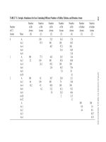
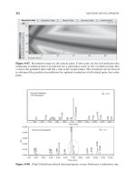
defined by equation (2-46).Typical experimental dependence of the minor dis-
turbance peak retention is shown in Figure 2-7.
Integration of function (2-46) allows the calculation of the excess adsorp-
tion values [22]:
(2-48)
Integration of this dependence through the whole concentration range actu-
ally allows the calculation of the column void volume, or the total volume of
the liquid phase in the column. Since excess adsorption of pure component is
equal to 0 (Γ(0) =Γ(100) = 0), then
(2-49)
Since the measurement of the excess adsorption isotherm of a component in
the binary system does not require a priori introduction of any model, it is
possible to consider the excess adsorption isotherm as being model-
independent (within a framework of adsorption process) and it is possible to
derive the properties of the adsorbed layer on the basis of consideration of
V
Vcdc
cc
R
c

c
0
0
100
0
0
=
()
−
=
=
∫
max
max
Γ c
S
VVdc
R
c
()
=−
()
∫
1
0
0
44 HPLC THEORY
Figure 2-7. Minor disturbance peak retention dependence as the function of the ace-
tonitrile concentration in water.