Tài liệu High Performance Computing on Vector Systems-P5 doc

The Role of Supercomputing in Industrial Combustion Modeling 115
parameter sweep. The control block is the program object which allows the
changing of the sequence of execution operation according to a specified criterion.
Figure 2 shows an example of task flow. After execution of “Task” block 1.1,
block 2.1 and block 3.1 are activated simultaneously. In each of these blocks
a process is executed. After having worked with the first set of data in block 1.1,
the first process in block 1.2 is activated. After execution of the first process in
block 1.2, the first process in block 1.3 and the second process in block 1.1 are
started according to the logic of the experiment. The input data for the second
and the following processes in block 1.1 are prepared in block 1.2 and so on.
3.2 Data Flow Level
Figure 3 presents an example of a solver block (Block 1.1). At this level, the user
can describe the manipulation of data in a very fine grained way. The solver block
consists of computation (C), replacement (R), parameterization (P) modules and
a database. These are connected to each other with arrowed lines showing the
direction of data transfer between modules and the sequence of execution during
the computation process.
Each module is a Java object, which has a standard structure and consists
of several sections. For example: each computation module (C) consists of four
sections. The first section organizes the preparation of input data. The second
generates the job and controls its execution. The third initializes and controls
the record of the result in the experiment database. The fourth section controls
the execution of module operation. It also informs the main program of the
block about the manipulation of certain sets of data and when execution within
a block is complete.
After a block is started, the parameterization module (P) and replacement
module (R) wait for the request from the corresponding inputs of the computa-
tion module (C). After that, they generate a set of input data according to rules
specified by the user, either as mathematical formulae or a list of parameter
values. In this example three variants of parameterization are represented:
(a) Direct transmission of the parameter values with the job. In this case, pa-

rameterization module (P3) transfers the generated parameter value to the
computation module (C1) upon its request. The computation module gen-
erates the job, including converting parameter values into corresponding job
parameters. This method can be used if the parameterized value is a number,
symbol or combination of both.
(b) Parameterized objects are large arrays of information (DB-P4 in Fig. 3) which
are kept in the experiment database. These parameters are copied directly
from the experiment database to the corresponding file server and then writ-
ten with the same array name with the index of the number of the stage.
In this case, attributes of the job are sent to the file server as references (an
array of data).
(c) If it is important, then the preparation of the data is moved outside of the
main program. This allows the creation of a more universal computation
Please purchase PDF Split-Merge on www.verypdf.com to remove this watermark.
116 N. Currle-Linde et al.
Fig. 3. Solver Block 1.1 (data flow)
module. Furthermore, it allows scaling, i.e. avoiding limitations in the size,
position, type and number of the parameterized objects used in a module.
In these cases the replacement module is used. During the preparation of the
next set of input data, new parameter values P1 and P2 are generated. The
generated parameter set is linked with replacement processes and then delivered
to the corresponding FileServer, where the replacement process is executed.
After the replacement of the specified parameters, the input data is ready
for the first stage of computation. Computation module C1 sends a message to
the JobManager to prepare the job for the first stage. The JobManager chooses
the computer resources currently available in the network and starts the job.
After confirmation from the corresponding SubServer of the Target Machine
that the job is in a queue, the preparation of the next set of data for the next
computation stage begins. Each new stage carries out the same processes as the
previous stage. At all stages, the output file is archived immediately after being

received by the experiment’s database. The control of all processes takes place
according to the pattern described above. After starting the ExpMonitorVIS
on their workstation, the user receives continuously updated status information
regarding the experiment’s progress.
4 Use case: Power Plant Simulation by Varying Burners
and Fuel Quality
The liberalization of the energy markets puts more and more pressure on the
competitiveness of power companies throughout the world. In order to maintain
Please purchase PDF Split-Merge on www.verypdf.com to remove this watermark.
The Role of Supercomputing in Industrial Combustion Modeling 117
their competitive edge, it is necessary to optimize the operation of existing power
plants towards minimum operational costs. Potential optimization targets can
be minimization of excess air (increasing efficiency) or NOx-emission (reducing
DeNOx operation costs). Pure experimental optimizations without computer-
aided techniques are time-consuming and require a significantly higher manpower
effort. Furthermore, in the case of necessary design changes the technical risks
involved in the investment decision can only be assessed with computer-aided
techniques. Computer-aided methods are well accepted in the power industry.
The optimization procedure applied by SEGL for the present problem is based
on a genetic algorithm (GA).
In order to work on boiler optimization problems with SEGL, the parameters
that have to be optimized are coded in binary form and assembled to a so-
called “chromosome”. The chromosome carries all the important properties to
be changed of the so-called “individuals”. A certain number of these artificial
individuals are generated initially, the so-called “population”, and the GA of
SEGL imitates the natural evolution process. The imitation is done by applying
the genetic mechanisms Selection, Recombination and Mutation. An illustration
of the basic workflow in the SEGL is shown in Fig. 4.
The basic workflow can be described as follows:
1. Binary coding of optimization parameters and chromosome assembly.

2. Generation of an initial population.
3. Decoding of the chromosome information for each individual.
Fig. 4. Workflow
Please purchase PDF Split-Merge on www.verypdf.com to remove this watermark.
118 N. Currle-Linde et al.
4. Simulation of the decoded set of optimization parameters with the 3D-
furnace simulation code RECOM-AIOLOS for each individual. This is the
time consuming step.
5. Filtering the 3-D results of the furnace simulation to derive the target values
for each individual.
6. Evaluation of the performance level for each individual (terminate the opti-
mization process if desired optimization level is reached).
7. Selection of suitable individuals for reproduction and Recombination/Muta-
tion of the chromosome information for the selected individuals to generate
new individuals.
8. Return to Step 3 for new individuals.
4.1 Industrial Applicability
An experimental operation optimization exercise performed in 1991 at a power
station in Italy (ENEL’s coal-fired Fusina) is used to demonstrate the capabilities
of SEGL. In a windbox, the amount of air flowing through a nozzle is controlled
by the damper setting of the nozzle. A damper setting of 100% means that the
flow passage of the nozzle is fully open. Reducing the damper setting of a single
nozzle allows for reduction of the air mass flow through the nozzle, but at the
same time the air mass flows for all other nozzles in the windbox are increased.
Fig. 5. Firing and separate OFA arrangement fur Fusina #2
Please purchase PDF Split-Merge on www.verypdf.com to remove this watermark.
The Role of Supercomputing in Industrial Combustion Modeling 119
In 1991 separate overfire air nozzles (separate OFA) were installed above the
main combustion zone (see Fig. 4) to minimize NOx-emissions. A new operation
mode was required after the successful installation of the separate overfire air to

maintain the lowest possible NOx-emission together with a minimum unburned
carbon loss. In 1991 this optimization exercise was solved experimentally. In
a series of 15 tests over a duration of approximately 10 days, 15 operation modes
were tested with varying amounts of close coupled overfire air (CCOFA), separate
OFA, and tilting angle of the separate OFA (±30
◦
).
The following operation experience was recorded to identify an optimized
operation:
(a) For a horizontal orientation of the separate OFA the maximum NOx-
reduction is reached with dampers 100% open.
(b) A tilting of the separate OFA to −30
◦
has a minor effect on the NOx-emission
but improves the burnout (reduced unburned carbon loss).
(c) A tilting of the separate OFA to +30
◦
leads to an NOx-reduction but in-
creases the unburned carbon loss significantly.
(d) Closing the CCOFA completely at 100% open separate OFA has only a minor
effect on the NOx-emission.
In order to work on this combustion optimization problem in virtual reality,
a high-resolution boiler model with 1 million grid points was generated. As shown
in Table 1, an accuracy of approximately ±10% between simulation and reality
can be reached on the high-resolution boiler model. The optimization param-
eters “OFA damper setting”, “CCOFA damper setting”, and “Tilting Angle”
Fig. 6. Evaluation functions for a NOx versus C in Ash optimization
Please purchase PDF Split-Merge on www.verypdf.com to remove this watermark.
120 N. Currle-Linde et al.
Table 1. Measured and calculated NOx-emission and C in Ash

NOx-emission [mg/m
3
n
,6%O
2
] CinAsh[%]
Setting measured calculated measured calculated
No OFA 950–966 954 6.41–7.50 5.66
No CCOFA
No OFA 847–858 794 7.47–7.61 6.58
CCOFA: 100%
OFA:100% 410–413 457 10.43–11.48 10.28
CCOFA: 100%
Table 2. Development of best individuals in each generation during automatic opti-
mization
Generation Target-Value OFA CCOFA Tilting Angle NOx CinAsh[%]
[%] [%] [
◦
] mg/m
3
n
Basis 12.070 0 0 0 805 3.39
1 10.061 100 100 −30 479 10.84
5 9.600 93 93 −30 473 10.42
10 9.177 93 20 −30 458 10.26
were coded with 4 bit on the chromosomes. NOx-emission and C in Ash values
achieved in the model were combined to a target function for the evaluation of
the individuals. The underlying combined evaluation target function are shown
in Fig. 6.
Target Function = Evaluation[NOx] + Evaluation[CinAsh]

The GA required approximately 11 generations with 10 individuals per popu-
lation to identify an optimized parameter set. During the course of the automatic
optimization, approximately 51 of the entire 4096 (2
4
· 2
4
· 2
4
) coded combina-
tions of parameter settings were evaluated with respect to the target functions.
Table 2 shows the development of the best individuals in each generation in the
course of the automatic optimization. The results demonstrate that SEGL is
able to identify the same positive measures that were found in the experimental
optimization. The final run on the high-resolution boiler model led to an NOx-
emission of 476 mg/m
3
n
at 6% O
2
and a C in Ash value of 8.42%. Both values
are in the range of the emission and C in Ash values that were observed in the
field after the optimization exercise.
4.2 Computational Performance of RECOM-AIOLOS
As well as accuracy, investigated in the previous section, computational economy
is an important requirement in the industrial use of 3D-combustion simulations.
The aim is to obtain solutions of acceptable accuracy within short time periods
and at low financial costs.
Please purchase PDF Split-Merge on www.verypdf.com to remove this watermark.
The Role of Supercomputing in Industrial Combustion Modeling 121
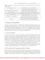
Table 3. Computational performance on varying number of processors and problem

size
Problem size Processors Gas combustion Solid Fuel combustion
5Mio.Gridpoints 1 processor 6.3 GFlops 4.3 GFlops
1Mio.Gridpoints 1 node=8 processors 24.9 GFlops 17.2 GFlops
5Mio.Gridpoints 1 node=8 processors 30.7 GFlops 21.2 GFlops
10 Mio. Grid points 1 node=8 processors 36.4 GFlops 25.1 GFlops
10 Mio. Grid points 4 node=64 processors 122.2 GFlops 84.3 GFlops
In order to exploit the possibilities of parallel execution RECOM-AIOLOS
has successfully been parallelized in the past with two different strategies: a do-
main decomposition method using MPI (Message Passing Interface) as the mes-
sage passing environment [7] and a data parallel approach using Microtasking [8].
These investigations were performed either on distributed memory massively
parallel computers (MPPs) or pure shared memory vector computers (PVPs),
showing acceptable parallel efficiencies for both approaches.
The architecture used in the present paper is a 72-node NEC SX-8 with
an aggregate peak-performance of 12 TFlops and a shared main memory of
9.2 TB. The NEC SX-8 supports a hybrid parallel programming model that
allows combination of distributed memory parallelization across nodes and data
parallel execution with the node.
The degree of vectorization of AIOLOS hereby defined as the ratio between
the time spent in the vector unit and the total user time is greater than 99.7%
depending on the problem size.
Table 3 shows the computational performance on varying number of proces-
sors and problem size. The results indicate that the code achieves 39% of the
theoretical single processor peak performance of 16 GFlops for the gas combus-
tion model. In the case of the solid fuel combustion model, only 27% of the single
processor peak performance is reached.
The total duration of the automatic optimization described in the previous
chapter was 3 days. The total optimisation consumed 581 CPUh.
5Conclusion

This paper presented the concept and description of the implementation of SEGL
for the design of complex and hierarchical parameter studies which offers an
efficient way to execute scientific experiments. We can show that SEGL allows
for substantial reduction in optimization costs for parameter studies.
This is a prerequisite for applying automatic optimization techniques to in-
dustrial combustion problems that will require hundreds of variations to be run
within today’s project time frames to derive practical conclusions for indus-
trial combustion equipment. High performance computers are helpful for this
purpose but high aggregated machine performance alone is not enough. Tools
Please purchase PDF Split-Merge on www.verypdf.com to remove this watermark.
122 N. Currle-Linde et al.
will be needed for managing virtual tests and the immense amount of data the
simulations produce. This will allow for an automated data handling and post-
processing.
References
1. de Vivo, A., Yarrow, M., McCann, K.: A comparison of parameter study creation
and job submission tools. Technical report, NASA Ames Research Center (2000)
2. Erwin, D.E.: Joint project report for the BMBF project UNICORE plus. Grant
Number: 01 IR 001 A-D, Duration: January 2000 – December 2002 (2003)
3. Taylor, I., Shields, M., Wangand, I., Philp, R.: Distributed P2P computing within
triana: A galaxy visualization test case. In: IPDPS 2003 Conference. (2003)
4. Tony, A., Curbera, F., Dholakia, H., Goland, Y., Klein, J., Leymann, F., Liu, K.,
Roller, D., Smith, D., Thatte, S., Trickovic, I., Weerawarana, S.: Specification:
Business process execution language for web services version 1.1. Technical report,
NASA Ames Research Center (2003)
5. Corporation, V.: Fastobject webpage. (2005)
6. Foster, I., Kesselman, C.: The globus project: A status report. In: Proc. IPPS/SPDP
’98 Heterogeneous Computing Workshop. (1998)
7. Lepper, J., Schnell, U., Hein, K.R.G.: Numerical simulation of large-scale combus-
tion processes on distributed memory parallel computers using mpi. In: Parallel

CFD 96. (1996)
8. Risio, B., Schnell, U., Hein, K.R.G.: HPF-implementation of a 3D-combustion code
on parallel computer architectures using fine grain parallelism. In: Parallel CFD 96.
(1996)
Please purchase PDF Split-Merge on www.verypdf.com to remove this watermark.
Simulation of the Unsteady Flow Field
Around a Complete Helicopter
with a Structured RANS Solver
Thorsten Schwarz, Walid Khier, and Jochen Raddatz
German Aerospace Center (DLR),
Member of the Helmholtz Association,
Institute of Aerodynamics and Flow Technology,
Lilienthalplatz 7, D-38108 Braunschweig, Germany

WWW home page: />Abstract The air flow past a wind tunnel model of an Eurocopter BO-105 fuselage,
main rotor and tail rotor configuration is simulated by solving the time dependent
Navier-Stokes equations. The flow solver uses overlapping, block structured grids to
discretize the computational domain. The simulation setup and the execution on a par-
allel NEC SX-6 vector computer are described. The numerical results are compared
with unsteady pressure measurements on the fuselage and the blades. An overall good
agreement is found. Differences between predicted and measured data on the main
rotor and the tail rotor can be explained by blade elasticity effects and a different trim
law respectively. The computational performance of the flow solver is analyzed for the
NEC SX-6 and NEC SX-8 vector computer showing a good parallel performance. Mod-
ifications of the code structure resulted in a reduction of the execution time for the
Chimera procedure by a factor of 6.6.
1 Introduction
The numerical simulation of the flow around a complete helicopter by solving
the unsteady Reynolds-averaged Navier-Stokes (RANS) equations is a challenge.
This is mainly due to a lack of available computer resources. The complex flow

topology around the helicopter and the unsteadiness of the flow requires com-
putations on grids with millions of grid cells and several thousand physical time
steps to solve the governing equations. Only today’s supercomputers are fast
enough and have enough memory to enable these kind of simulations within
a research context. Another issue for helicopter simulations is fluid modeling,
e.g. vortex capturing and turbulence modeling.
The flow field around a helicopter is depicted in Fig. 1. A helicopter usually
operates at flight speeds below M =0.3. Therefore, the flow is incompressible
except for the regions near the blade tips of the main and tail rotor where the
Please purchase PDF Split-Merge on www.verypdf.com to remove this watermark.
126 T. Schwarz, W. Khier, J. Raddatz
blade−vortex
interaction
tip
vortex
fuselage−vortex
in
teraction
tailrotor−vortex
interaction
shock
infl
ow
flow separation
dynamic
stall
Fig. 1. Aerodynamics of the helicopter
flow may be locally supersonic and shocks may be present. Strong vortices are
shed from the blade tips and move downstream with the inflow velocity. These
vortices can interact with the following blades. The viscosity of the fluid leads

to boundary layers on surfaces and wake sheets downstream of the surfaces. The
boundary layers may separate at bluff body components. Flow separation may
also occur at the retreating rotor blades, where due to trim considerations the
blade incidence angle must be high. Additionally, interactions take place between
the helicopter’s components, e.g. between the main-rotor, the tail-rotor and the
fuselage. All the aforementioned phenomena affect the flight performance of the
helicopter, its vibration and its noise emission.
Since flow simulations for complete helicopters are not possible in an indus-
trial environment, the solution of the Navier-Stokes equations is often restricted
to individual components of a helicopter. Examples are steady flow simulations
for isolated fuselages [1] or unsteady simulations for isolated main rotors [2, 3, 4].
Interactional phenomena between the rotors and the fuselage have been investi-
gated with steady flow simulations, where the main and tail rotors are replaced
by actuator discs [5]. The latter are used to prescribe the time averaged effects of
the rotors. First Navier-Stokes computations for a full helicopter configuration
have been presented in [6, 7, 8].
In an effort to provide the French-German helicopter manufacturer Euro-
copter with simulation tools capable of computing the viscous flow around com-
plete helicopters, the project CHANCE [9, 10] was initiated in 1999. Project
partners have been the German and French research centers DLR and ONERA,
the university of Stuttgart and the helicopter manufacturer Eurocopter. Within
the CHANCE project, the flow solvers of DLR and ONERA have been widely ex-
tended and were validated for helicopter flows. One final milestone of the project
was to simulate the unsteady flow for a complete helicopter configuration. The
aim of this paper is to present results obtained by DLR with the block-structured
flow solver FLOWer for such a configuration.
Please purchase PDF Split-Merge on www.verypdf.com to remove this watermark.
Flow Simulation for Complete Helicopter 127
2 Simulated Test Case and Flow Conditions
The computations reported here simulate a forward flight test case of a 1:2.5

scale wind tunnel model of an Eurocopter BO-105. The wind tunnel experiment
was performed within the EU project HeliNOVI [11] in 2003. (Please note, that
most of the HeliNOVI experiments were performed during a second campaign in
2004). Figure 2 shows the model mounted on a model support inside the German-
Dutch wind tunnel (DNW). The BO-105 wind tunnel model has a main rotor
diameter of 4 m and a tail rotor diameter equal to 0.773 m. Both the main and
tail rotors have square blades. The main rotor blades consist of −8
◦
linearly
twisted NACA 23012 profile with a chord length equal to 0.121 m. The tail rotor
is made of a MBB S 102 E airfoil with zero twist and has a chord length equal
to 0.0733 m. All intake and ventilation openings were closed in the experimental
model. A cylindrical strut was used to support the model in the wind tunnel. The
experimental model, its instrumentation and the wind tunnel tests are described
in detail by [12].
Fig. 2. BO-105 wind tunnel model
The selected test case refers to a forward flight condition with 60 m/s (M =
0.177) at an angle of attack equal to 5.2
◦
. The main and tail rotor angular
velocities are equal to 1085 and 5304 RPM respectively, corresponding to a main
rotor tip Mach number M
ωR
MR
=0.652 and a tail rotor tip Mach number
M
ωR
TR
=0.63. The nominal trim law for the main and tail rotor blade pitch
angles used in the experiment was Θ

MR
=10.5
◦
−6.3
◦
sin(Ψ
MR
)+1.9
◦
cos(Ψ
MR
)
forthemainrotorandΘ
TR
=8.0
◦
for the tail rotor. Ψ
MR
is the azimuth angle
of the main rotor. Information on the flapping and elastic blade deformation of
the main rotor were not available at the time of the simulation. The same holds
for the coupled cyclic pitching/flapping motion of the tail rotor.
Please purchase PDF Split-Merge on www.verypdf.com to remove this watermark.
128 T. Schwarz, W. Khier, J. Raddatz
3 Numerical Approach
DLR’s flow solver FLOWer solves the Reynolds-averaged Navier-Stokes equa-
tions with a second order accurate finite volume discretization on structured,
multi-block grids. The solution process follows the idea of Jameson [13], who
represents the mass, momentum and energy fluxes by second order central dif-
ferences. Third order numerical dissipation is added to the convective fluxes to

ensure numerical stability.
FLOWer contains a large array of statistical turbulence models, ranging from
algebraic and one-equation eddy viscosity models to seven-equation Reynolds
stress models. In this paper a slightly modified version of Wilcox’s two-equation
k-ω model is used [14, 15]. Unlike the main flow equations, Roe’s scheme is
employed to compute the turbulent convective fluxes.
For steady flows, the discretized equations are advanced in time using an ex-
plicit five-stage Runge-Kutta method. The solution process makes use of acceler-
ation techniques like local time stepping, multigrid and implicit residual smooth-
ing. Turbulence transport equations are integrated implicitly with a DDADI
(diagonal dominant alternating direction implicit) method. For unsteady simu-
lations, the implicit dual time stepping method [16, 17] is applied. FLOWer is
parallelized based on MPI and is optimized for vector computers.
A method extensively used within the present work is the Chimera overlap-
ping grid technique [18]. This method allows to discretize the computational
domain with a set of overlapping grids, see Fig. 3. In order to establish com-
munication between the grids, data from overlapping grids are interpolated for
the cells at the outer grid boundaries. If some grid points are positioned inside
solid bodies, these points are flagged and are not considered during the flow
simulations. The flagged points form a so called hole in the grid. At the hole
fringe, data are interpolated from overlapping grids. A detailed description of
the Chimera method implemented in FLOWer is given in [19].
The Chimera technique is used in the present computations because of the
following reasons. Firstly, compared to alternative approaches (re-meshing for
example), relative motion between the different components of the helicopter
background grid
component grid
hole
fringe cells
outer Chimera

boundary
Fig. 3. The Chimera technique, left: overlapping grids, right: interpolation points
Please purchase PDF Split-Merge on www.verypdf.com to remove this watermark.