Tài liệu 31 Channel Equalization as a Regularized Inverse Problem doc
Bạn đang xem bản rút gọn của tài liệu. Xem và tải ngay bản đầy đủ của tài liệu tại đây (196.64 KB, 10 trang )
Doherty, J.F. “Channel Equalization as a Regularized Inverse Problem”
Digital Signal Processing Handbook
Ed. Vijay K. Madisetti and Douglas B. Williams
Boca Raton: CRC Press LLC, 1999
c
1999byCRCPressLLC
31
Channel Equalization as a
Regularized Inverse Problem
John F. Doherty
Pennsylvania State University
31.1 Introduction
31.2 Discrete-Time Intersymbol Interference Channel Model
31.3 Channel Equalization Filtering
Matrix Formulation of the Equalization Problem
31.4 Regularization
31.5 Discrete-Time Adaptive Filtering
Adaptive Algorithm Recapitulation
•
Regularization Proper-
ties of Adaptive Algorithms
31.6 Numerical Results
31.7 Conclusion
References
31.1 Introduction
In this article we examine the problem of communication channel equalization and how it relates
to the inversion of a linear system of equations. Channel equalization is the process by which the
effect of a band-limited channel may be diminished, i.e., equalized, at the sink of a communication
system. Although there are many ways to accomplish this, we will concentrate on linear filters and
adaptive filters. It is through the linear filter approach that the analogy to matrix inversion is possible.
Regularized inversion refers to a process in which noise dominated modes of the observed signal are
attenuated.
31.2 Discrete-Time Intersymbol Interference Channel Model
Intersymbol interference (ISI) is a phenomenon observed by the equalizer caused by frequency
distortion of the transmitted signal. This distortion is usually caused by the frequency selective
characteristics of the transmission medium. However, it can also be due to deliberate time dispersion
of the transmitted pulse to affect realizable implementations of the transmit filter. In any case, the
purpose of the equalizer is to remove deleterious effects of the ISI on symbol detection. The ISI
generation mechanism is described next with a description of equalization techniques to follow. The
information transmitted by a digital communication system is comprised of a set of discrete symbols.
Likewise, the ultimate form of the received information is cast into a discrete form. However, the
intermediate components of the digital communications system operate with continuous waveforms
which carry the information. The major portions of the communications link are the transmitter
c
1999 by CRC Press LLC
pulse shaping filter, the modulator, the channel, the demodulator, and the receiver filter. It will be
advantageous to transform the continuous part of the communication system into an equivalent
discrete time channel description for simulation purposes. The discrete formulation should be
transparent to both the information source and the equalizer when evaluating performance. The
equivalent discrete time channel model is attained by combining the transmit filter, p(t), the channel
filter, g(t), and the receive filter, w(t), into a single continuous filter, that is,
h(t) = w(t)∗ g(t)∗ p(t)
(31.1)
Refer to Fig. 31.1. The effect of the sampler preceding the decision device is to discretize the aggre-
FIGURE 31.1: The signal flow block diagram for the equivalent channel description. The equalizer
observes x(nT ), a sampled version of the receive filter output x(t).
gate filter. The equivalent discrete time channel as a means to simulate the performance of digital
communications systems was advanced by Proakis [1] and has found subsequent use throughout the
communications literature [2, 3].
It has been shown that a bandpass transmitted pulse train has an equivalent low pass representa-
tion [1]
s(t)=
∞
n=0
A
n
p(t − nT )
(31.2)
where
{
A
n
}
is the information bearing symbol set, p(t) is the equivalent low pass transmit pulse
waveform, and T is the symbol rate. The observed signal at the input of the receiver is
r(t) =
∞
n=0
A
n
+∞
−∞
p(t − nT )g(t − nT − τ)dτ + n(t)
(31.3)
where g(t) is the equivalent low pass bandlimited impulse response of the channel and the channel
noise, n(t), is modeled as white Gaussian noise. The optimum receiver filter, w(t), is the matched
filter which is designed to give maximum correlation with the received pulse [4]. The output of the
receiver filter, that is, the signal seen by the sampler, can be written as
x(t) =
∞
n=0
A
n
h(t − nT ) + ν(t)
(31.4)
h(t) =
+∞
−∞
+∞
−∞
p(t − nT )g(t − nT − λ)dλ
w(t − τ)dτ
(31.5)
ν(t) =
+∞
−∞
n(t)w(t − τ)dτ
(31.6)
where h(t) is the response of the receiver filter to the received pulse, representing the overall impulse
response between the transmitter and the sampler, and ν(t) =
+∞
−∞
n(t)w(t − τ)dτ is a filtered
c
1999 by CRC Press LLC
version of the channel noise. The input to the equalizer is a sampled version of Eq. (31.4), that is,
sampling at times t = kT produces
x(kT ) =
∞
n=0
A
n
h(kt − nT ) + ν(kT )
(31.7)
as the input to the discrete time equalizer. By normalizing with respect to the sampling interval and
rearranging terms, Eq. (31.7) becomes
x
k
= h
0
A
k
desired symbol
+
∞
n=0
n=k
A
n
h
k−n
intersymbol interference
+ ν
k
(31.8)
31.3 Channel Equalization Filtering
31.3.1 Matrix Formulation of the Equalization Problem
The task of finding the optimum linear equalizer coefficients can be described by casting the problem
into a system of linear equations,
˜
d
1
˜
d
2
.
.
.
˜
d
L
=
x
T
1
x
T
2
.
.
.
x
T
L
c +
e
1
e
2
.
.
.
e
L
(31.9)
x
k
=
x
k+N−1
,...,x
k−1
T
(31.10)
where (·)
T
denotes the transpose operation. The received sample at time k is x
k
, which consists of the
channel output corrupted by additive noise. The elements of the N × 1 vector c
k
are the coefficients
of the equalizer filter at time k. The equalizer is said to be in decision directed mode when
˜
d
k
is taken
as the output of the nonlinear decision device. The equalizer is in training, or reference directed,
mode when
˜
d
k
is explicitly made identical to the transmitted sequence A
k
. In either case, e
k
is the
error between the desired equalizer output,
˜
d
k
, and the actual equalizer output, x
T
k
c. We will assume
that
˜
d
k
= A
k+N
, then the notation in Eq. (31.9) can be written in the compact form,
d = Xc + e
(31.11)
by defining d =
˜
d
1
,...,
˜
d
L
T
and by making the obvious associations with Eq. (31.9). Note that
the parameter L determines the number of rows of the time varying matrix X. Therefore, choosing
L is analogous to choosing an observation interval for the estimation of the filter coefficients.
31.4 Regularization
We seek a solution for the filter coefficients of the form c = Yd,whereY is in some sense an inverse
of the data matrix X. The least squares solution requires that
Y =
X
T
X
−1
X
T
(31.12)
c
1999 by CRC Press LLC
where X
#
=
X
T
X
−1
X
T
represents the Moore-Penrose (M-P) inverse of X. If one or more of the
eigenvalues of the matrix X
T
X is zero, then the Moore-Penrose inverse does not exist.
To investigate the behavior of the inverse, we will decompose the data matrix into the form X =
X
S
+ X
N
,whereX
S
is the signal component and X
N
is the noise component. Generally, the noise
data matrix is full rank and the signal data matrix may be nearly rank deficient from the spectral
nulls in the transmission channel. This is illustrated by examining the smallest eigenvalue of X
T
S
X
S
λ
min
= S
R min
+ O
N
−k
(31.13)
where S
R
is the continuous PSD of the received data x
k
, S
R min
is the minimum value of the PSD, k
is the number of non-vanishing derivatives of S
R
at S
R min
, and N is the equalizer filter length. Any
spectral loss in the signal caused by the channel is directly translated into a corresponding decrease
in the minimum eigenvalue of the received signal. If λ
min
becomes small, but nonzero, the data
correlation matrix X
T
X becomes ill-conditioned and its inversion becomes sensitive to the noise.
The sensitivity is expressed in the quantity
δ
=
˜
c − c
c
≤
σ
2
n
λ
min
+ O
σ
4
n
(31.14)
where the noiseless least squares filter coefficient vector solution, c, has been perturbed by adding a
white noise to the data with variance σ
2
n
1, to produce the least squares solution
˜
c. Substituting
Eq. (31.13) into Eq. (31.14) yields
δ ≤
σ
2
n
S
R min
+ O
N
−k
+ O
σ
4
n
≈
σ
2
n
S
R min
(31.15)
The relation in Eq. (31.15) is an indicator of the potential numerical problems in solving for the
equalizer filter coefficients when the data is spectrally deficient.
We see that direct inversion of the data matrix is not recommendable when the channel has severe
spectral nulls. This situation is equivalent to stating that the original estimation problem d = Xc
is ill-posed. That is, the equalizer is asked to reproduce components of the channel input that are
unobservable at the channel output or are obscured by noise. Thus, it is reasonable to ascertain the
modes of the input dominated by noise and give them little weight, relative to the signal dominated
components, when solving for the equalizer filter coefficients. This process of weighting is called
regularization.
Regularization can be described by relying on a generalization of the M-P inverse that depends on
the singular value decomposition (SVD) of the data matrix
X = UV
T
(31.16)
where U is an L× N unitary matrix, V is an N × N unitary matrix, = diag
(
σ
1
,σ
2
,...,σ
N
)
is a
diagonal matrix of singular values where σ
i
≥ 0, σ
1
>σ
2
> ··· >σ
N
. It is assumed in Eq. (31.16)
that L>N, which is typical in the equalization problem.
We define the generalized pseudo-inverse of X as
X
†
= V
†
U
T
(31.17)
where
†
= diag
σ
†
1
,σ
†
2
,...,σ
†
N
and
σ
†
i
=
σ
−1
i
σ
i
= 0
0 σ
i
= 0
(31.18)
c
1999 by CRC Press LLC