Astrom murray feedback systems for scientists engineers txtbk

www.elsolucionario.net


www.elsolucionario.net


Feedback Systems

An Introduction for Scientists and Engineers

˚
Karl Johan Aström
Richard M. Murray

Version v2.10e (30 August 2011)
This is the electronic edition of Feedback Systems and is available
from Hardcover
editions may be purchased from Princeton Univeristy Press,
/>This manuscript is for personal use only and may not be
reproduced, in whole or in part, without written consent from the
publisher (see />
PRINCETON UNIVERSITY PRESS
PRINCETON AND OXFORD

www.elsolucionario.net


Copyright © 2008 by Princeton University Press
Published by Princeton University Press
41 William Street, Princeton, New Jersey 08540
In the United Kingdom: Princeton University Press

6 Oxford Street, Woodstock, Oxfordshire OX20 1TW
All Rights Reserved
Library of Congress Cataloging-in-Publication Data
Åström, Karl J. (Karl Johan), 1934Feedback systems : an introduction for scientists and engineers / Karl Johan
Åström and Richard M. Murray
p. cm.
Includes bibliographical references and index.
ISBN-13: 978-0-691-13576-2 (alk. paper)
ISBN-10: 0-691-13576-2 (alk. paper)
1. Feedback control systems. I. Murray, Richard M., 1963-. II. Title.
TJ216.A78 2008
629.8′ 3–dc22
2007061033
British Library Cataloging-in-Publication Data is available
This book has been composed in LATEX
The publisher would like to acknowledge the authors of this volume for providing
the camera-ready copy from which this book was printed.
Printed on acid-free paper. ∞
press.princeton.edu
Printed in the United States of America
10 9 8 7 6 5 4

www.elsolucionario.net


ii

This version of Feedback Systems is the electronic edition of the text. Revision
history:
• Version 2.10e (30 Aug 2011): electronic edition, with corrections

• Version 2.10d (19 Jul 2011): electronic edition, with corrections
• Version 2.10c (4 Mar 2010): third printing, with corrections
• Version 2.10b (22 Feb 2009): second printing, with corrections
• Version 2.10a (2 Dec 2008): electronic edition, with corrections
• Version 2.9d (30 Jan 2008): first printing
A full list of changes made in each revision is available on the companion web site:
/>
www.elsolucionario.net


Contents

Preface

vi

Chapter 1. Introduction
1.1 What Is Feedback?
1.2 What Is Control?
1.3 Feedback Examples
1.4 Feedback Properties
1.5 Simple Forms of Feedback
1.6 Further Reading
Exercises

1
1
3
5
17

23
25
26

Chapter 2. System Modeling
2.1 Modeling Concepts
2.2 State Space Models
2.3 Modeling Methodology
2.4 Modeling Examples
2.5 Further Reading
Exercises

27
27
34
44
51
61
61

Chapter 3. Examples
3.1 Cruise Control
3.2 Bicycle Dynamics
3.3 Operational Amplifier Circuits
3.4 Computing Systems and Networks
3.5 Atomic Force Microscopy
3.6 Drug Administration
3.7 Population Dynamics
Exercises

66
66
70
72
76
82
85
90
92

Chapter 4. Dynamic Behavior
4.1 Solving Differential Equations
4.2 Qualitative Analysis
4.3 Stability
4.4 Lyapunov Stability Analysis
4.5 Parametric and Nonlocal Behavior

96
96
99
103
111
121

www.elsolucionario.net


iv

CONTENTS

4.6

Further Reading
Exercises

127
127

Chapter 5. Linear Systems
5.1 Basic Definitions
5.2 The Matrix Exponential
5.3 Input/Output Response
5.4 Linearization
5.5 Further Reading
Exercises

132
132
137
146
159
164
165

Chapter 6. State Feedback
6.1 Reachability
6.2 Stabilization by State Feedback
6.3 State Feedback Design
6.4 Integral Action

6.5 Further Reading
Exercises

168
168
176
184
196
198
199

Chapter 7. Output Feedback
7.1 Observability
7.2 State Estimation
7.3 Control Using Estimated State
7.4 Kalman Filtering
7.5 A General Controller Structure
7.6 Further Reading
Exercises

202
202
207
212
216
220
227
227

Chapter 8. Transfer Functions

8.1 Frequency Domain Modeling
8.2 Derivation of the Transfer Function
8.3 Block Diagrams and Transfer Functions
8.4 The Bode Plot
8.5 Laplace Transforms
8.6 Further Reading
Exercises

230
230
232
243
251
260
263
263

Chapter 9. Frequency Domain Analysis
9.1 The Loop Transfer Function
9.2 The Nyquist Criterion
9.3 Stability Margins
9.4 Bode’s Relations and Minimum Phase Systems
9.5 Generalized Notions of Gain and Phase
9.6 Further Reading

269
269
272
280
285

287
292

www.elsolucionario.net


v

CONTENTS

Exercises

293

Chapter 10. PID Control
10.1 Basic Control Functions
10.2 Simple Controllers for Complex Systems
10.3 PID Tuning
10.4 Integrator Windup
10.5 Implementation
10.6 Further Reading
Exercises

296
296
301
305
309
311
316

316

Chapter 11. Frequency Domain Design
11.1 Sensitivity Functions
11.2 Feedforward Design
11.3 Performance Specifications
11.4 Feedback Design via Loop Shaping
11.5 Fundamental Limitations
11.6 Design Example
11.7 Further Reading
Exercises

319
319
323
326
330
335
344
347
348

Chapter 12. Robust Performance
12.1 Modeling Uncertainty
12.2 Stability in the Presence of Uncertainty
12.3 Performance in the Presence of Uncertainty
12.4 Robust Pole Placement
12.5 Design for Robust Performance
12.6 Further Reading
Exercises

351
351
356
362
365
373
378
378

Bibliography

381

Index

391

www.elsolucionario.net


Preface

This book provides an introduction to the basic principles and tools for the design
and analysis of feedback systems. It is intended to serve a diverse audience of
scientists and engineers who are interested in understanding and utilizing feedback
in physical, biological, information and social systems. We have attempted to keep
the mathematical prerequisites to a minimum while being careful not to sacrifice
rigor in the process. We have also attempted to make use of examples from a variety
of disciplines, illustrating the generality of many of the tools while at the same time

showing how they can be applied in specific application domains.
A major goal of this book is to present a concise and insightful view of the
current knowledge in feedback and control systems. The field of control started
by teaching everything that was known at the time and, as new knowledge was
acquired, additional courses were developed to cover new techniques. A consequence of this evolution is that introductory courses have remained the same for
many years, and it is often necessary to take many individual courses in order to
obtain a good perspective on the field. In developing this book, we have attempted
to condense the current knowledge by emphasizing fundamental concepts. We believe that it is important to understand why feedback is useful, to know the language
and basic mathematics of control and to grasp the key paradigms that have been
developed over the past half century. It is also important to be able to solve simple
feedback problems using back-of-the-envelope techniques, to recognize fundamental limitations and difficult control problems and to have a feel for available design
methods.
This book was originally developed for use in an experimental course at Caltech
involving students from a wide set of backgrounds. The course was offered to
undergraduates at the junior and senior levels in traditional engineering disciplines,
as well as first- and second-year graduate students in engineering and science. This
latter group included graduate students in biology, computer science and physics.
Over the course of several years, the text has been classroom tested at Caltech and
at Lund University, and the feedback from many students and colleagues has been
incorporated to help improve the readability and accessibility of the material.
Because of its intended audience, this book is organized in a slightly unusual
fashion compared to many other books on feedback and control. In particular, we
introduce a number of concepts in the text that are normally reserved for secondyear courses on control and hence often not available to students who are not
control systems majors. This has been done at the expense of certain traditional
topics, which we felt that the astute student could learn independently and are often

www.elsolucionario.net


vii

PREFACE

explored through the exercises. Examples of topics that we have included are nonlinear dynamics, Lyapunov stability analysis, the matrix exponential, reachability
and observability, and fundamental limits of performance and robustness. Topics
that we have deemphasized include root locus techniques, lead/lag compensation
and detailed rules for generating Bode and Nyquist plots by hand.
Several features of the book are designed to facilitate its dual function as a basic
engineering text and as an introduction for researchers in natural, information and
social sciences. The bulk of the material is intended to be used regardless of the
audience and covers the core principles and tools in the analysis and design of
feedback systems. Advanced sections, marked by the “dangerous bend” symbol
shown here, contain material that requires a slightly more technical background,
of the sort that would be expected of senior undergraduates in engineering. A few
sections are marked by two dangerous bend symbols and are intended for readers
with more specialized backgrounds, identified at the beginning of the section. To
limit the length of the text, several standard results and extensions are given in the
exercises, with appropriate hints toward their solutions.
To further augment the printed material contained here, a companion web site
has been developed and is available from the publisher’s web page:
/>The web site contains a database of frequently asked questions, supplemental examples and exercises, and lecture material for courses based on this text. The material is
organized by chapter and includes a summary of the major points in the text as well
as links to external resources. The web site also contains the source code for many
examples in the book, as well as utilities to implement the techniques described in
the text. Most of the code was originally written using MATLAB M-files but was
also tested with LabView MathScript to ensure compatibility with both packages.
Many files can also be run using other scripting languages such as Octave, SciLab,
SysQuake and Xmath.
The first half of the book focuses almost exclusively on state space control
systems. We begin in Chapter 2 with a description of modeling of physical, biological and information systems using ordinary differential equations and difference

equations. Chapter 3 presents a number of examples in some detail, primarily as a
reference for problems that will be used throughout the text. Following this, Chapter 4 looks at the dynamic behavior of models, including definitions of stability
and more complicated nonlinear behavior. We provide advanced sections in this
chapter on Lyapunov stability analysis because we find that it is useful in a broad
array of applications and is frequently a topic that is not introduced until later in
one’s studies.
The remaining three chapters of the first half of the book focus on linear systems,
beginning with a description of input/output behavior in Chapter 5. In Chapter 6,
we formally introduce feedback systems by demonstrating how state space control
laws can be designed. This is followed in Chapter 7 by material on output feedback and estimators. Chapters 6 and 7 introduce the key concepts of reachability

www.elsolucionario.net


viii

PREFACE

and observability, which give tremendous insight into the choice of actuators and
sensors, whether for engineered or natural systems.
The second half of the book presents material that is often considered to be
from the field of “classical control.” This includes the transfer function, introduced
in Chapter 8, which is a fundamental tool for understanding feedback systems.
Using transfer functions, one can begin to analyze the stability of feedback systems
using frequency domain analysis, including the ability to reason about the closed
loop behavior of a system from its open loop characteristics. This is the subject of
Chapter 9, which revolves around the Nyquist stability criterion.
In Chapters 10 and 11, we again look at the design problem, focusing first
on proportional-integral-derivative (PID) controllers and then on the more general
process of loop shaping. PID control is by far the most common design technique

in control systems and a useful tool for any student. The chapter on frequency
domain design introduces many of the ideas of modern control theory, including
the sensitivity function. In Chapter 12, we combine the results from the second half
of the book to analyze some of the fundamental trade-offs between robustness and
performance. This is also a key chapter illustrating the power of the techniques that
have been developed and serving as an introduction for more advanced studies.
The book is designed for use in a 10- to 15-week course in feedback systems
that provides many of the key concepts needed in a variety of disciplines. For a
10-week course, Chapters 1–2, 4–6 and 8–11 can each be covered in a week’s time,
with the omission of some topics from the final chapters. A more leisurely course,
spread out over 14–15 weeks, could cover the entire book, with 2 weeks on modeling
(Chapters 2 and 3)—particularly for students without much background in ordinary
differential equations—and 2 weeks on robust performance (Chapter 12).
The mathematical prerequisites for the book are modest and in keeping with
our goal of providing an introduction that serves a broad audience. We assume
familiarity with the basic tools of linear algebra, including matrices, vectors and
eigenvalues. These are typically covered in a sophomore-level course on the subject, and the textbooks by Apostol [Apo69], Arnold [Arn87] and Strang [Str88]
can serve as good references. Similarly, we assume basic knowledge of differential
equations, including the concepts of homogeneous and particular solutions for linear ordinary differential equations in one variable. Apostol [Apo69] and Boyce and
DiPrima [BD04] cover this material well. Finally, we also make use of complex
numbers and functions and, in some of the advanced sections, more detailed concepts in complex variables that are typically covered in a junior-level engineering or
physics course in mathematical methods. Apostol [Apo67] or Stewart [Ste02] can
be used for the basic material, with Ahlfors [Ahl66], Marsden and Hoffman [MH98]
or Saff and Snider [SS02] being good references for the more advanced material.
We have chosen not to include appendices summarizing these various topics since
there are a number of good books available.
One additional choice that we felt was important was the decision not to rely
on a knowledge of Laplace transforms in the book. While their use is by far the
most common approach to teaching feedback systems in engineering, many stu-

www.elsolucionario.net


ix

PREFACE

dents in the natural and information sciences may lack the necessary mathematical
background. Since Laplace transforms are not required in any essential way, we
have included them only in an advanced section intended to tie things together
for students with that background. Of course, we make tremendous use of transfer
functions, which we introduce through the notion of response to exponential inputs,
an approach we feel is more accessible to a broad array of scientists and engineers.
For classes in which students have already had Laplace transforms, it should be
quite natural to build on this background in the appropriate sections of the text.
Acknowledgments
The authors would like to thank the many people who helped during the preparation
of this book. The idea for writing this book came in part from a report on future
directions in control [Mur03] to which Stephen Boyd, Roger Brockett, John Doyle
and Gunter Stein were major contributors. Kristi Morgansen and Hideo Mabuchi
helped teach early versions of the course at Caltech on which much of the text is
based, and Steve Waydo served as the head TA for the course taught at Caltech in
2003–2004 and provided numerous comments and corrections. Charlotta Johnsson and Anton Cervin taught from early versions of the manuscript in Lund in
2003–2007 and gave very useful feedback. Other colleagues and students who provided feedback and advice include Leif Andersson, John Carson, K. Mani Chandy,
Michel Charpentier, Domitilla Del Vecchio, Kate Galloway, Per Hagander, Toivo
Henningsson Perby, Joseph Hellerstein, George Hines, Tore Hägglund, Cole Lepine, Anders Rantzer, Anders Robertsson, Dawn Tilbury and Francisco Zabala. The
reviewers for Princeton University Press and Tom Robbins at NI Press also provided
valuable comments that significantly improved the organization, layout and focus
of the book. Our editor, Vickie Kearn, was a great source of encouragement and help
throughout the publishing process. Finally, we would like to thank Caltech, Lund

University and the University of California at Santa Barbara for providing many
resources, stimulating colleagues and students, and pleasant working environments
that greatly aided in the writing of this book.
Karl Johan Åström
Lund, Sweden
Santa Barbara, California

Richard M. Murray
Pasadena, California

www.elsolucionario.net


Chapter One
Introduction
Feedback is a central feature of life. The process of feedback governs how we grow, respond
to stress and challenge, and regulate factors such as body temperature, blood pressure and
cholesterol level. The mechanisms operate at every level, from the interaction of proteins in
cells to the interaction of organisms in complex ecologies.
M. B. Hoagland and B. Dodson, The Way Life Works, 1995 [HD95].

In this chapter we provide an introduction to the basic concept of feedback and
the related engineering discipline of control. We focus on both historical and current
examples, with the intention of providing the context for current tools in feedback
and control. Much of the material in this chapter is adapted from [Mur03], and
the authors gratefully acknowledge the contributions of Roger Brockett and Gunter
Stein to portions of this chapter.

1.1 What Is Feedback?
A dynamical system is a system whose behavior changes over time, often in response

to external stimulation or forcing. The term feedback refers to a situation in which
two (or more) dynamical systems are connected together such that each system
influences the other and their dynamics are thus strongly coupled. Simple causal
reasoning about a feedback system is difficult because the first system influences
the second and the second system influences the first, leading to a circular argument.
This makes reasoning based on cause and effect tricky, and it is necessary to analyze
the system as a whole. A consequence of this is that the behavior of feedback systems
is often counterintuitive, and it is therefore necessary to resort to formal methods
to understand them.
Figure 1.1 illustrates in block diagram form the idea of feedback. We often use
the terms open loop and closed loop when referring to such systems. A system
is said to be a closed loop system if the systems are interconnected in a cycle, as
shown in Figure 1.1a. If we break the interconnection, we refer to the configuration
as an open loop system, as shown in Figure 1.1b.
As the quote at the beginning of this chapter illustrates, a major source of examples of feedback systems is biology. Biological systems make use of feedback in an
extraordinary number of ways, on scales ranging from molecules to cells to organisms to ecosystems. One example is the regulation of glucose in the bloodstream
through the production of insulin and glucagon by the pancreas. The body attempts
to maintain a constant concentration of glucose, which is used by the body’s cells
to produce energy. When glucose levels rise (after eating a meal, for example), the

www.elsolucionario.net


2

1.1. WHAT IS FEEDBACK?

u
System 1

y
System 2

(a) Closed loop

r

u
System 1

y
System 2

(b) Open loop

Figure 1.1: Open and closed loop systems. (a) The output of system 1 is used as the input of
system 2, and the output of system 2 becomes the input of system 1, creating a closed loop
system. (b) The interconnection between system 2 and system 1 is removed, and the system
is said to be open loop.

hormone insulin is released and causes the body to store excess glucose in the liver.
When glucose levels are low, the pancreas secretes the hormone glucagon, which
has the opposite effect. Referring to Figure 1.1, we can view the liver as system 1
and the pancreas as system 2. The output from the liver is the glucose concentration
in the blood, and the output from the pancreas is the amount of insulin or glucagon
produced. The interplay between insulin and glucagon secretions throughout the
day helps to keep the blood-glucose concentration constant, at about 90 mg per
100 mL of blood.
An early engineering example of a feedback system is a centrifugal governor,
in which the shaft of a steam engine is connected to a flyball mechanism that is

itself connected to the throttle of the steam engine, as illustrated in Figure 1.2. The
system is designed so that as the speed of the engine increases (perhaps because of a
lessening of the load on the engine), the flyballs spread apart and a linkage causes the
throttle on the steam engine to be closed. This in turn slows down the engine, which
causes the flyballs to come back together. We can model this system as a closed
loop system by taking system 1 as the steam engine and system 2 as the governor.
When properly designed, the flyball governor maintains a constant speed of the
engine, roughly independent of the loading conditions. The centrifugal governor
was an enabler of the successful Watt steam engine, which fueled the industrial
revolution.
Feedback has many interesting properties that can be exploited in designing
systems. As in the case of glucose regulation or the flyball governor, feedback can
make a system resilient toward external influences. It can also be used to create linear
behavior out of nonlinear components, a common approach in electronics. More
generally, feedback allows a system to be insensitive both to external disturbances
and to variations in its individual elements.
Feedback has potential disadvantages as well. It can create dynamic instabilities
in a system, causing oscillations or even runaway behavior. Another drawback,
especially in engineering systems, is that feedback can introduce unwanted sensor
noise into the system, requiring careful filtering of signals. It is for these reasons
that a substantial portion of the study of feedback systems is devoted to developing
an understanding of dynamics and a mastery of techniques in dynamical systems.
Feedback systems are ubiquitous in both natural and engineered systems. Con-

www.elsolucionario.net


3

1.2. WHAT IS CONTROL?

Figure 1.2: The centrifugal governor and the steam engine. The centrifugal governor on the
left consists of a set of flyballs that spread apart as the speed of the engine increases. The
steam engine on the right uses a centrifugal governor (above and to the left of the flywheel)
to regulate its speed. (Credit: Machine a Vapeur Horizontale de Philip Taylor [1828].)

trol systems maintain the environment, lighting and power in our buildings and
factories; they regulate the operation of our cars, consumer electronics and manufacturing processes; they enable our transportation and communications systems;
and they are critical elements in our military and space systems. For the most part
they are hidden from view, buried within the code of embedded microprocessors,
executing their functions accurately and reliably. Feedback has also made it possible to increase dramatically the precision of instruments such as atomic force
microscopes (AFMs) and telescopes.
In nature, homeostasis in biological systems maintains thermal, chemical and
biological conditions through feedback. At the other end of the size scale, global
climate dynamics depend on the feedback interactions between the atmosphere, the
oceans, the land and the sun. Ecosystems are filled with examples of feedback due
to the complex interactions between animal and plant life. Even the dynamics of
economies are based on the feedback between individuals and corporations through
markets and the exchange of goods and services.

1.2 What Is Control?
The term control has many meanings and often varies between communities. In
this book, we define control to be the use of algorithms and feedback in engineered
systems. Thus, control includes such examples as feedback loops in electronic amplifiers, setpoint controllers in chemical and materials processing, “fly-by-wire”
systems on aircraft and even router protocols that control traffic flow on the Internet. Emerging applications include high-confidence software systems, autonomous
vehicles and robots, real-time resource management systems and biologically engineered systems. At its core, control is an information science and includes the

www.elsolucionario.net

4

1.2. WHAT IS CONTROL?

noise

external disturbances

Actuators

System

noise

Output

Sensors
Process

Clock

D/A

Computer

A/D

Filter
Controller

operator input
Figure 1.3: Components of a computer-controlled system. The upper dashed box represents
the process dynamics, which include the sensors and actuators in addition to the dynamical
system being controlled. Noise and external disturbances can perturb the dynamics of the
process. The controller is shown in the lower dashed box. It consists of a filter and analog-todigital (A/D) and digital-to-analog (D/A) converters, as well as a computer that implements
the control algorithm. A system clock controls the operation of the controller, synchronizing
the A/D, D/A and computing processes. The operator input is also fed to the computer as an
external input.

use of information in both analog and digital representations.
A modern controller senses the operation of a system, compares it against the
desired behavior, computes corrective actions based on a model of the system’s
response to external inputs and actuates the system to effect the desired change.
This basic feedback loop of sensing, computation and actuation is the central concept in control. The key issues in designing control logic are ensuring that the
dynamics of the closed loop system are stable (bounded disturbances give bounded
errors) and that they have additional desired behavior (good disturbance attenuation, fast responsiveness to changes in operating point, etc). These properties are
established using a variety of modeling and analysis techniques that capture the
essential dynamics of the system and permit the exploration of possible behaviors
in the presence of uncertainty, noise and component failure.
A typical example of a control system is shown in Figure 1.3. The basic elements
of sensing, computation and actuation are clearly seen. In modern control systems,
computation is typically implemented on a digital computer, requiring the use of
analog-to-digital (A/D) and digital-to-analog (D/A) converters. Uncertainty enters
the system through noise in sensing and actuation subsystems, external disturbances
that affect the underlying system operation and uncertain dynamics in the system
(parameter errors, unmodeled effects, etc). The algorithm that computes the control
action as a function of the sensor values is often called a control law. The system
can be influenced externally by an operator who introduces command signals to

www.elsolucionario.net

5

1.3. FEEDBACK EXAMPLES

the system.
Control engineering relies on and shares tools from physics (dynamics and
modeling), computer science (information and software) and operations research
(optimization, probability theory and game theory), but it is also different from
these subjects in both insights and approach.
Perhaps the strongest area of overlap between control and other disciplines is in
the modeling of physical systems, which is common across all areas of engineering
and science. One of the fundamental differences between control-oriented modeling and modeling in other disciplines is the way in which interactions between
subsystems are represented. Control relies on a type of input/output modeling that
allows many new insights into the behavior of systems, such as disturbance attenuation and stable interconnection. Model reduction, where a simpler (lower-fidelity)
description of the dynamics is derived from a high-fidelity model, is also naturally
described in an input/output framework. Perhaps most importantly, modeling in a
control context allows the design of robust interconnections between subsystems,
a feature that is crucial in the operation of all large engineered systems.
Control is also closely associated with computer science since virtually all modern control algorithms for engineering systems are implemented in software. However, control algorithms and software can be very different from traditional computer software because of the central role of the dynamics of the system and the
real-time nature of the implementation.

1.3 Feedback Examples
Feedback has many interesting and useful properties. It makes it possible to design
precise systems from imprecise components and to make relevant quantities in a
system change in a prescribed fashion. An unstable system can be stabilized using
feedback, and the effects of external disturbances can be reduced. Feedback also
offers new degrees of freedom to a designer by exploiting sensing, actuation and
computation. In this section we survey some of the important applications and

trends for feedback in the world around us.
Early Technological Examples
The proliferation of control in engineered systems occurred primarily in the latter
half of the 20th century. There are some important exceptions, such as the centrifugal
governor described earlier and the thermostat (Figure 1.4a), designed at the turn of
the century to regulate the temperature of buildings.
The thermostat, in particular, is a simple example of feedback control that everyone is familiar with. The device measures the temperature in a building, compares
that temperature to a desired setpoint and uses the feedback error between the two
to operate the heating plant, e.g., to turn heat on when the temperature is too low
and to turn it off when the temperature is too high. This explanation captures the
essence of feedback, but it is a bit too simple even for a basic device such as the

www.elsolucionario.net


6

1.3. FEEDBACK EXAMPLES

Movement
opens
throttle

Load
Spring

Latch
Electromagnet

Reversible

Motor

(a) Honeywell thermostat, 1953

Accelerator
Pedal
SpeedAdjustment
Knob
Governor
Contacts
Latching
Button
Flyball
SpeedGovernor
ometer
Adjustment
Spring

(b) Chrysler cruise control, 1958

Figure 1.4: Early control devices. (a) Honeywell T87 thermostat originally introduced in
1953. The thermostat controls whether a heater is turned on by comparing the current temperature in a room to a desired value that is set using a dial. (b) Chrysler cruise control system
introduced in the 1958 Chrysler Imperial [Row58]. A centrifugal governor is used to detect
the speed of the vehicle and actuate the throttle. The reference speed is specified through an
adjustment spring. (Left figure courtesy of Honeywell International, Inc.)

thermostat. Because lags and delays exist in the heating plant and sensor, a good
thermostat does a bit of anticipation, turning the heater off before the error actually
changes sign. This avoids excessive temperature swings and cycling of the heating
plant. This interplay between the dynamics of the process and the operation of the

controller is a key element in modern control systems design.
There are many other control system examples that have developed over the
years with progressively increasing levels of sophistication. An early system with
broad public exposure was the cruise control option introduced on automobiles in
1958 (see Figure 1.4b). Cruise control illustrates the dynamic behavior of closed
loop feedback systems in action—the slowdown error as the system climbs a grade,
the gradual reduction of that error due to integral action in the controller, the small
overshoot at the top of the climb, etc. Later control systems on automobiles such
as emission controls and fuel-metering systems have achieved major reductions of
pollutants and increases in fuel economy.
Power Generation and Transmission
Access to electrical power has been one of the major drivers of technological
progress in modern society. Much of the early development of control was driven
by the generation and distribution of electrical power. Control is mission critical
for power systems, and there are many control loops in individual power stations.
Control is also important for the operation of the whole power network since it
is difficult to store energy and it is thus necessary to match production to consumption. Power management is a straightforward regulation problem for a system
with one generator and one power consumer, but it is more difficult in a highly

www.elsolucionario.net


7

1.3. FEEDBACK EXAMPLES

Figure 1.5: A small portion of the European power network. By 2008 European power
suppliers will operate a single interconnected network covering a region from the Arctic to
the Mediterranean and from the Atlantic to the Urals. In 2004 the installed power was more
than 700 GW (7 × 1011 W). (Source: UCTE [www.ucte.org])

distributed system with many generators and long distances between consumption
and generation. Power demand can change rapidly in an unpredictable manner and
combining generators and consumers into large networks makes it possible to share
loads among many suppliers and to average consumption among many customers.
Large transcontinental and transnational power systems have therefore been built,
such as the one show in Figure 1.5.
Most electricity is distributed by alternating current (AC) because the transmission voltage can be changed with small power losses using transformers. Alternating
current generators can deliver power only if the generators are synchronized to the
voltage variations in the network. This means that the rotors of all generators in a
network must be synchronized. To achieve this with local decentralized controllers
and a small amount of interaction is a challenging problem. Sporadic low-frequency
oscillations between distant regions have been observed when regional power grids
have been interconnected [KW05].
Safety and reliability are major concerns in power systems. There may be disturbances due to trees falling down on power lines, lightning or equipment failures.
There are sophisticated control systems that attempt to keep the system operating
even when there are large disturbances. The control actions can be to reduce voltage, to break up the net into subnets or to switch off lines and power users. These
safety systems are an essential element of power distribution systems, but in spite
of all precautions there are occasionally failures in large power systems. The power
system is thus a nice example of a complicated distributed system where control is
executed on many levels and in many different ways.

www.elsolucionario.net


8

1.3. FEEDBACK EXAMPLES

(a) F/A-18 “Hornet”

(b) X-45 UCAV

Figure 1.6: Military aerospace systems. (a) The F/A-18 aircraft is one of the first production
military fighters to use “fly-by-wire” technology. (b) The X-45 (UCAV) unmanned aerial
vehicle is capable of autonomous flight, using inertial measurement sensors and the global
positioning system (GPS) to monitor its position relative to a desired trajectory. (Photographs
courtesy of NASA Dryden Flight Research Center.)

Aerospace and Transportation
In aerospace, control has been a key technological capability tracing back to the
beginning of the 20th century. Indeed, the Wright brothers are correctly famous
not for demonstrating simply powered flight but controlled powered flight. Their
early Wright Flyer incorporated moving control surfaces (vertical fins and canards)
and warpable wings that allowed the pilot to regulate the aircraft’s flight. In fact,
the aircraft itself was not stable, so continuous pilot corrections were mandatory.
This early example of controlled flight was followed by a fascinating success story
of continuous improvements in flight control technology, culminating in the highperformance, highly reliable automatic flight control systems we see in modern
commercial and military aircraft today (Figure 1.6).
Similar success stories for control technology have occurred in many other
application areas. Early World War II bombsights and fire control servo systems
have evolved into today’s highly accurate radar-guided guns and precision-guided
weapons. Early failure-prone space missions have evolved into routine launch operations, manned landings on the moon, permanently manned space stations, robotic
vehicles roving Mars, orbiting vehicles at the outer planets and a host of commercial and military satellites serving various surveillance, communication, navigation
and earth observation needs. Cars have advanced from manually tuned mechanical/pneumatic technology to computer-controlled operation of all major functions,
including fuel injection, emission control, cruise control, braking and cabin comfort.
Current research in aerospace and transportation systems is investigating the
application of feedback to higher levels of decision making, including logical regulation of operating modes, vehicle configurations, payload configurations and health
status. These have historically been performed by human operators, but today that

www.elsolucionario.net


9

1.3. FEEDBACK EXAMPLES

Figure 1.7: Materials processing. Modern materials are processed under carefully controlled
conditions, using reactors such as the metal organic chemical vapor deposition (MOCVD)
reactor shown on the left, which was for manufacturing superconducting thin films. Using
lithography, chemical etching, vapor deposition and other techniques, complex devices can
be built, such as the IBM cell processor shown on the right. (MOCVD image courtesy of Bob
Kee. IBM cell processor photograph courtesy Tom Way, IBM Corporation; unauthorized use
not permitted.)

boundary is moving and control systems are increasingly taking on these functions.
Another dramatic trend on the horizon is the use of large collections of distributed
entities with local computation, global communication connections, little regularity
imposed by the laws of physics and no possibility of imposing centralized control
actions. Examples of this trend include the national airspace management problem,
automated highway and traffic management and command and control for future
battlefields.
Materials and Processing
The chemical industry is responsible for the remarkable progress in developing
new materials that are key to our modern society. In addition to the continuing need
to improve product quality, several other factors in the process control industry
are drivers for the use of control. Environmental statutes continue to place stricter
limitations on the production of pollutants, forcing the use of sophisticated pollution
control devices. Environmental safety considerations have led to the design of
smaller storage capacities to diminish the risk of major chemical leakage, requiring

tighter control on upstream processes and, in some cases, supply chains. And large
increases in energy costs have encouraged engineers to design plants that are highly
integrated, coupling many processes that used to operate independently. All of these
trends increase the complexity of these processes and the performance requirements
for the control systems, making control system design increasingly challenging.
Some examples of materials-processing technology are shown in Figure 1.7.
As in many other application areas, new sensor technology is creating new
opportunities for control. Online sensors—including laser backscattering, video

www.elsolucionario.net


10

1.3. FEEDBACK EXAMPLES

microscopy and ultraviolet, infrared and Raman spectroscopy—are becoming more
robust and less expensive and are appearing in more manufacturing processes. Many
of these sensors are already being used by current process control systems, but
more sophisticated signal-processing and control techniques are needed to use more
effectively the real-time information provided by these sensors. Control engineers
also contribute to the design of even better sensors, which are still needed, for
example, in the microelectronics industry. As elsewhere, the challenge is making
use of the large amounts of data provided by these new sensors in an effective
manner. In addition, a control-oriented approach to modeling the essential physics
of the underlying processes is required to understand the fundamental limits on
observability of the internal state through sensor data.
Instrumentation
The measurement of physical variables is of prime interest in science and engineering. Consider, for example, an accelerometer, where early instruments consisted of
a mass suspended on a spring with a deflection sensor. The precision of such an

instrument depends critically on accurate calibration of the spring and the sensor.
There is also a design compromise because a weak spring gives high sensitivity but
low bandwidth.
A different way of measuring acceleration is to use force feedback. The spring
is replaced by a voice coil that is controlled so that the mass remains at a constant
position. The acceleration is proportional to the current through the voice coil. In
such an instrument, the precision depends entirely on the calibration of the voice coil
and does not depend on the sensor, which is used only as the feedback signal. The
sensitivity/bandwidth compromise is also avoided. This way of using feedback has
been applied to many different engineering fields and has resulted in instruments
with dramatically improved performance. Force feedback is also used in haptic
devices for manual control.
Another important application of feedback is in instrumentation for biological
systems. Feedback is widely used to measure ion currents in cells using a device
called a voltage clamp, which is illustrated in Figure 1.8. Hodgkin and Huxley used
the voltage clamp to investigate propagation of action potentials in the giant axon
of the squid. In 1963 they shared the Nobel Prize in Medicine with Eccles for “their
discoveries concerning the ionic mechanisms involved in excitation and inhibition
in the peripheral and central portions of the nerve cell membrane.” A refinement of
the voltage clamp called a patch clamp made it possible to measure exactly when a
single ion channel is opened or closed. This was developed by Neher and Sakmann,
who received the 1991 Nobel Prize in Medicine “for their discoveries concerning
the function of single ion channels in cells.”
There are many other interesting and useful applications of feedback in scientific instruments. The development of the mass spectrometer is an early example.
In a 1935 paper, Nier observed that the deflection of ions depends on both the
magnetic and the electric fields [Nie35]. Instead of keeping both fields constant,
Nier let the magnetic field fluctuate and the electric field was controlled to keep the

www.elsolucionario.net

11

1.3. FEEDBACK EXAMPLES

Electrode
∆vr
Controller

Glass Pipette
Ion Channel

I

ve vi +

∆v

Cell Membrane
Figure 1.8: The voltage clamp method for measuring ion currents in cells using feedback. A
pipet is used to place an electrode in a cell (left and middle) and maintain the potential of the
cell at a fixed level. The internal voltage in the cell is v i , and the voltage of the external fluid
is v e . The feedback system (right) controls the current I into the cell so that the voltage drop
across the cell membrane v = v i − v e is equal to its reference value vr . The current I is
then equal to the ion current.

ratio between the fields constant. Feedback was implemented using vacuum tube
amplifiers. This scheme was crucial for the development of mass spectroscopy.
The Dutch engineer van der Meer invented a clever way to use feedback to
maintain a good-quality high-density beam in a particle accelerator [MPTvdM80].

The idea is to sense particle displacement at one point in the accelerator and apply
a correcting signal at another point. This scheme, called stochastic cooling, was
awarded the Nobel Prize in Physics in 1984. The method was essential for the
successful experiments at CERN where the existence of the particles W and Z
associated with the weak force was first demonstrated.
The 1986 Nobel Prize in Physics—awarded to Binnig and Rohrer for their design
of the scanning tunneling microscope—is another example of an innovative use of
feedback. The key idea is to move a narrow tip on a cantilever beam across a surface
and to register the forces on the tip [BR86]. The deflection of the tip is measured
using tunneling. The tunneling current is used by a feedback system to control the
position of the cantilever base so that the tunneling current is constant, an example
of force feedback. The accuracy is so high that individual atoms can be registered.
A map of the atoms is obtained by moving the base of the cantilever horizontally.
The performance of the control system is directly reflected in the image quality and
scanning speed. This example is described in additional detail in Chapter 3.
Robotics and Intelligent Machines
The goal of cybernetic engineering, already articulated in the 1940s and even before,
has been to implement systems capable of exhibiting highly flexible or “intelligent”
responses to changing circumstances. In 1948 the MIT mathematician Norbert
Wiener gave a widely read account of cybernetics [Wie48]. A more mathematical
treatment of the elements of engineering cybernetics was presented by H. S. Tsien
in 1954, driven by problems related to the control of missiles [Tsi54]. Together,
these works and others of that time form much of the intellectual basis for modern
work in robotics and control.
Two accomplishments that demonstrate the successes of the field are the Mars

www.elsolucionario.net


12

1.3. FEEDBACK EXAMPLES

Figure 1.9: Robotic systems. (a) Spirit, one of the two Mars Exploratory Rovers that landed on
Mars in January 2004. (b) The Sony AIBO Entertainment Robot, one of the first entertainment
robots to be mass-marketed. Both robots make use of feedback between sensors, actuators and
computation to function in unknown environments. (Photographs courtesy of Jet Propulsion
Laboratory and Sony Electronics, Inc.)

Exploratory Rovers and entertainment robots such as the Sony AIBO, shown in
Figure 1.9. The two Mars Exploratory Rovers, launched by the Jet Propulsion
Laboratory (JPL), maneuvered on the surface of Mars for more than 4 years starting
in January 2004 and sent back pictures and measurements of their environment. The
Sony AIBO robot debuted in June 1999 and was the first “entertainment” robot to be
mass-marketed by a major international corporation. It was particularly noteworthy
because of its use of artificial intelligence (AI) technologies that allowed it to act in
response to external stimulation and its own judgment. This higher level of feedback
is a key element in robotics, where issues such as obstacle avoidance, goal seeking,
learning and autonomy are prevalent.
Despite the enormous progress in robotics over the last half-century, in many
ways the field is still in its infancy. Today’s robots still exhibit simple behaviors
compared with humans, and their ability to locomote, interpret complex sensory
inputs, perform higher-level reasoning and cooperate together in teams is limited.
Indeed, much of Wiener’s vision for robotics and intelligent machines remains
unrealized. While advances are needed in many fields to achieve this vision—
including advances in sensing, actuation and energy storage—the opportunity to
combine the advances of the AI community in planning, adaptation and learning
with the techniques in the control community for modeling, analysis and design of
feedback systems presents a renewed path for progress.
Networks and Computing Systems

Control of networks is a large research area spanning many topics, including congestion control, routing, data caching and power management. Several features of
these control problems make them very challenging. The dominant feature is the
extremely large scale of the system; the Internet is probably the largest feedback

www.elsolucionario.net


13

1.3. FEEDBACK EXAMPLES

Clients

The Internet

Request

Request

Request

Reply

Reply

Reply

Tier 1

Tier 2

Tier 3

(a) Multitiered Internet services

(b) Individual server

Figure 1.10: A multitier system for services on the Internet. In the complete system shown
schematically in (a), users request information from a set of computers (tier 1), which in turn
collect information from other computers (tiers 2 and 3). The individual server shown in (b)
has a set of reference parameters set by a (human) system operator, with feedback used to
maintain the operation of the system in the presence of uncertainty. (Based on Hellerstein et
al. [HDPT04].)

control system humans have ever built. Another is the decentralized nature of the
control problem: decisions must be made quickly and based only on local information. Stability is complicated by the presence of varying time lags, as information
about the network state can be observed or relayed to controllers only after a delay,
and the effect of a local control action can be felt throughout the network only after
substantial delay. Uncertainty and variation in the network, through network topology, transmission channel characteristics, traffic demand and available resources,
may change constantly and unpredictably. Other complicating issues are the diverse
traffic characteristics—in terms of arrival statistics at both the packet and flow time
scales—and the different requirements for quality of service that the network must
support.
Related to the control of networks is control of the servers that sit on these networks. Computers are key components of the systems of routers, web servers and
database servers used for communication, electronic commerce, advertising and
information storage. While hardware costs for computing have decreased dramatically, the cost of operating these systems has increased because of the difficulty in
managing and maintaining these complex interconnected systems. The situation is
similar to the early phases of process control when feedback was first introduced to
control industrial processes. As in process control, there are interesting possibilities for increasing performance and decreasing costs by applying feedback. Several
promising uses of feedback in the operation of computer systems are described in

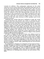
the book by Hellerstein et al. [HDPT04].
A typical example of a multilayer system for e-commerce is shown in Figure 1.10a. The system has several tiers of servers. The edge server accepts incoming requests and routes them to the HTTP server tier where they are parsed and
distributed to the application servers. The processing for different requests can vary
widely, and the application servers may also access external servers managed by
other organizations.
Control of an individual server in a layer is illustrated in Figure 1.10b. A quan-

www.elsolucionario.net