A comparison of real and simulated designs for vibratory parts feeding

A Comparison of Real and Simulated Designs for Vibratory Parts Feeding
Dina R. Berkowitz

John Canny


Department of Electrical Engineering and Computer Science
University of California, Berkeley, CA 94720
Abstract
The design of industrial parts feeders is a long, trial-and-
error process that can take months – even for the design
of feeders that orient only one type of part. This paper
describes the use of dynamic simulation to expedite the
design and prototyping of parts feeders. We give proba-
bilistic descriptions of vibratory parts feeding behavior, and
we present a comparison between simulated design experi-
ments and physical experiments done using a real industrial
vibratory bowl feeder. Our findings show strong similarities
between the results of the two types of experiments. We be-
lieve that dynamic simulation is a promising approach for
expediting the parts feeder analysis and design process.
1 Introduction
Although the vibratory parts feeders used in industry to
sort and orient parts are quite reliable, their design is time-
consuming. This is largely due to the trial-and-error nature
of the design process. We wouldliketo use dynamic simula-
tiontoexpeditetheefficientand effectivedesign ofindustrial
parts feeders.
In our previous work, we described a tool to automati-
cally generate, perform, and evaluate suites of feeder design
experimentsusing dynamic simulation

[
1
]
. In that workand
here we used Mirtich’s impulse-based dynamic simulator,
Impulse
[
11; 12
]
.
Impulse usesa friction-based modeltosimulatethe micro-
collisions occurring between impacting bodies. A previous
paper by Mirtich et al. gives results suggesting that Impulse
can predict the dynamical interactions found in industrial
parts feeding tasks
[
13
]
. Preliminary findings from our
former work also suggest that dynamic simulation may be
a promising approach for designing parts feeders. In this
paper, we discuss results from our current parts feeding
experiments.
The primary contribution of this paper is to compare the
experimental results from designs we have simulated using
dynamic simulation to those of an actual vibratory bowl.
We show the accuracy of Impulse’s simulation results by
comparing them to an actual vibratory bowl feeder using
real industrial parts.


Financial support provided by National Science Foundation
Grant #FD93-19412.
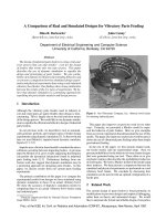
Figure 1: Our Vibromatic Company, Inc. vibratory bowl feeder
for orienting industrial parts.
This paper also improves on previous work in two other
ways. Formerly, we presented a Markov model to repre-
sent the behavior of parts feeders. Here we give examples
from our recent experiments that demonstrate the use of this
model. The paper also improvesonpreviousworkbecause it
shows the use of vibrational parts feeding rather than simple
gravitational feeding.
In the rest of the paper, we first present related work,
our feeder model, and our experimental setup. Next we
presentprobabilitiesfor the behaviorof some feeder designs
that were generated using our tool. These allow us to give
stochastic matrices that describe the probabilistic behaviors
of feedergates. We forma Markovmodelof the feeder using
these matrices. We then present a comparison between the
simulated and physical experiments we performed on a real
vibratory bowl feeder. We conclude by discussing how
simulation can be used to find an optimal configuration of a
feeder gate.
2 Related Work
The current design of parts feeders is based primarily on
modifications to previous designs and empirical debugging,
rather than on theory and automated design. We would
like to automate the formal and reliable design of sensorless
Proc. of the IEEE Int. Conf. on Robotics and Automation (ICRA’97), Albuquerque, New Mexico, April 1997.
parts feeders. We use dynamic simulation to address the
parts feeder design problem. A number of researchers have

investigated this problem and related problems analytically.
Boothroydand his colleagues, Murch and Poli, developed
a taxonomy of industrial parts and corresponding feeders
for orienting them. Their work was seminal in examining
geometricaland physicalconsiderations of the feederdesign
problem
[
3; 14
]
.
The tool we developed previously, enables us to auto-
matically generate and perform many experiments over a
parameterized multidimensional space of potential designs
[
1
]
. In a similar manner, Brost parameterized an operation
space of grasping motions for producing a desired outcome.
His algorithm incorporated uncertainty to guarantee suc-
cessful operations. He implemented and tested his planner
successfully using a real manipulator
[
5
]
.
Natarajan introduced several formal paradigms for de-
signing sensorless parts feeders
[
15
]

. Erdmann, Mason, and
Van
ˇ
e
ˇ
cek developeda sensorless table-tilting planner for ori-
enting three-dimensional polyhedral parts
[
7
]
. These two
papers, along with the description of the Markov model
in our previous work, propose modelling the parts feeding
problem using state transitions.
Others have developed analytical methods to uniquely
orient singulated parts being fed in a stream. Goldberg de-
scribed a planning algorithm and automatic programmable
parts feeder that can orient parts rapidly by analyzing their
geometry
[
8
]
. Brokowski, Peshkin, and Goldberg proposed
the use of curved fences above a moving conveyorto orient
streams of parts
[
4
]
.
Research in the past few years has included the devel-

opment of sensorless strategies to manipulate parts using
vibratory motion. B
¨
ohringer, Bhatt, and Goldberg exam-
ined the use of changing dynamic modes of a vibrating plate
to orient parts sitting on the plate
[
2
]
. Christiansen, Ed-
wards, and Coello Coello developed a genetic algorithm
that searches for optimal designs of vibratory bowl feed-
ers
[
6
]
. Our system generates the feeder gate probabilities
required by their algorithm as input.
More recently, researchershavecompared estimates from
analytical methods to physical experiments in the industrial
parts feeding domain. Mirtich et al. presented a system-
atic comparison of quasi-static algorithmic and Monte Carlo
simulated approaches to physical experiments
[
13
]
. Krish-
nasamy, Jakiela, and Whitney analyzed vibration-assisted
entrapment of both simulatedand physicalexperiments
[

10
]
.
Reznik, Brown, and Canny presented a qualitative exami-
nation of micro-actuated motion arrays based on dynamic
simulation and physical results
[
16
]
. In this paper, we com-
pare simulated and real designs for vibratory parts feeding.
3 Modelling And Experimental Setup
To run physical and simulatedvibratoryfeedingexperiments
“side-by-side”, we developed models of a vibratory bowl
feeder and parts by using measurements takenfrom an actual
Figure 2: Industrial parts for vibratory feeding and orienting.
Medium-sized parts are shown in the foreground and tall-sized
parts are shown in the background.
industrial vibratory bowl and the parts it was designed to
orient.
The feeder we used is a vibratory bowl feeder manufac-
tured by Vibromatic Company, Inc. (see Figure 1). We used
tall- and medium-sized cylindrical parts in our experiments.
The actual parts are cylindrical shells or sleeves that are
made of stainless steel wire mesh covered with aluminum
foil. The cylindrical sleeves are actual parts that are used in
the automotive industry (see Figure 2).
3.1 Vibratory Motion
A vibratory bowl’s oscillating leaf springs cause a con-
strained motion of torsional vibration about the feeder’s ver-

tical axis coupled with translational vibration in its vertical
direction.
The resulting motion of parts at any point on the bowl’s
horizontal track is along a line determined by the bowl’s
vibration angle

and amplitude
A
. The amplitude controls
how big the vibrational motions are, or how much energy is
put into the system (see Figure 3).
Horizontal
Track
Direction of Vibration
A
Ay
Ax
ψ
Figure 3: Motion of the track floor in a vibratory bowl, where
A
x
and
A
y
are the horizontal and vertical components of the amplitude
A
, respectively, and

is the vibration angle.
When the bowl feeder is operating properly, the vertical

component of itsamplitude will be thesame at everylocation
in the bowl. The horizontal component of vibration varies
linearly with the distance from the bowl’s axis of rotation.
3.2 Feeder Description
The Vibromatic, Inc. feeder we used to executeour physical
experiments is approximately 23 inches high and 32 inches
Proc. of the IEEE Int. Conf. on Robotics and Automation (ICRA’97), Albuquerque, New Mexico, April 1997.
z
x
y
Direction
of Motion
UT
UB
CT
CB
LT
LB
Figure 4: The six cylinder orientations – Upright Top (UT), Up-
right Bottom (UB), Crosswise Top (CT), Crosswise Bottom (CB),
Lengthwise Top (LT), Lengthwise Bottom (LB) – feeding across
the Slope gate (figure to scale).
in diameter. It has a mass of about 750 pounds and includes
a stainless-steel hopper bowl that weighs about 250 pounds
(see Figure 1). A reconfigurable vibratory bowl feeder of
this nature and size costs approximately $8500.
The bowl is mounted to a steel base drive unit. Four sets
of leaf springs are attached to the base. Two electromagnetic
coils attached to the base cause the leaf springs to oscillate
at 60 Hertz, delivering 60 vibrational mechanical motions

to the bowl per second. The amplitude of these vibrations
is adjustable.
The bowlitself has reconfigurable selectors, or gates, that
are located at various points along the bowl’s helical track.
The different sections of track preceding and following the
gates have varying positive and negative values of pitch.
Additionally, the track has varying inward and outward roll.
The gates along the track can be easily reconfigured for a
number of discrete settings (through the use of thumb-type
screws for making the adjustment).
3.3 Part Modelling
We model the cylindrical sleeves as solid, many-faceted
cylinders of uniform size and mass. However, the actual
cylinders vary in size and mass from part to part. For each
cylinder size, we thus modelled the mass, height, and diam-
eter by taking the median of each of the dimensions from
a sampling of the bulk parts. In our models the mid- and
tall-sized cylinders have diameters of 3.0 cm, heights of 2.5
and 3.7 cm, and masses of 9 and 12.5 grams, respectively
(see Figure 2). We measured the dimensions and masses of
the parts manually using rulers and mass balances.
We decomposed the state space of possible stable cylin-
der orientations into three equivalenceclasses: Upright (U),
Crosswise (C), and Lengthwise (L). However, some parts
flip 180 degrees in the course of feeding through the gate,
so we found it useful to further subdivide each of these into
two classes called Top (T) and Bottom (B). To distinguish
between the subclasses, we imagine painting a ring around
one end of each cylinder. This gives us a total of six classes,
labelled UT, UB, CT, CB, LT, and LB, respectively (see Fig-

ure 4). To account for radial symmetry about the cylinder’s
major axis, each equivalence class consists of twelve states
formed by rotating the part about its major axis in thirty
degree increments.
3.4 Simulated Designs
We model a vibratory bowl feeder as a single straight track
formed by unravelling the bowl’s helical track. As long
as a feeder’s gates are far enough apart not to interact, we
can study their effects in isolation
[
14
]
. Simulating each
gate with our tool independently allows us to compute the
probabilityfor each pre- and post-orientation of the gate that
one will be converted into the other.
Although the actual bowl has several different gates, in
this work we simulate and study one particular gate, Slope
(see Figure4). Slope can be reconfiguredtohavevarious an-
gles of decline. It is designed to turn Lengthwise parts onto
their ends, and to allow Upright parts to pass unchanged.
At the gate’s sub-optimal settings, it reorients few parts into
their upright orientations and knocks most upright parts into
the lengthwise orientations.
Our simulations model the physical bowl feeder’s fixed
and varying parameters. Our geometrical model is based on
dimension and angle measurements we took of the feeder
using rulers and protractors. From these measurements,
we approximated the bowl’s vibration angle and amplitude,
track angle, and gate dimensions. Since determining the vi-

bration amplitude was difficult, we simulated two amplitude
values in our experiments.
All the centers of mass and moments of inertia of the
objects in the simulations are computed automatically by
Impulse, based on the objects’ geometrical models.
We referenced a standard chart (which lists friction coef-
ficients for common materials) in a physics text to choose
the coefficient of friction. To determine the coefficient of
restitution, we attempted to observe the actual part’s inter-
action with the physical feeder. However, since this was
somewhat difficult, we also varied restitution over a small
range of values in our simulations.
The tool we developed previously enables us to auto-
matically generate and perform many experiments over a
multidimensional space of potential designs. It automati-
cally generates the multiple design experiments by taking
the Cartesian product over all the parameter values. It also
allows us to specify equivalence classes of stable states, and
it then automatically categorizes the state (and hence, the
equivalence class) of each part as the part exits the gate.
4 Experimental Results
All of the resultscollectedfor thephysical bowlexperiments
were observed and recorded by a human observer. For each
of the three initial stable orientations, Crosswise (CT), Up-
right (UT), and Lengthwise (LT), we observed 500 trials of
Proc. of the IEEE Int. Conf. on Robotics and Automation (ICRA’97), Albuquerque, New Mexico, April 1997.
Init
C U L
C U L
U

e
0.17
e
0.47
e
0.36
G1
1.0
G1
0.81
G1
0.19
G1
0.81
G1
0.19
G2
1.0
G2
1.0
G2
1.0
Gate 1
Transitions
Gate 2
Transitions
Figure 5: Markov model representing two consecutive gates,
Slope and Discharge Chute (labelled G1 and G2), in our simu-
lated vibratory bowl feeder for the mid-sized cylinders. Gate 1
was simulated with Slope = 12

:
8

, Amplitude = 0.06 cm, and
Restitution = 0.4. The epsilon (e) probabilities and the Gate 2
probabilities were taken from the actual feeder data.
singulated (non-interacting) parts moving across the Slope
gate. We observed physical experiments for each of the
two-sized parts with the angle of Slope set to 12.8 degrees
and a measured vibration angle of 15 degrees (see Figure 3).
For the simulations, we varied the feeder’s coefficient of
restitution and vibration amplitude. In particular, we ex-
perimented with restitution values ranging over the interval

0
:
3
;
0
:
5
]
in step sizes of 0.1, and we examined vibration
amplitudes of 0.06 and 0.1 cm. Each experiment consisted
of a suite of 500 trials for a fixed set of parameter values for
each of the three initial part orientations.
4.1 Markov Model Development
We represent the effects produced by the feeder’s gates as
state transitions in a non-deterministicfinite state automaton
(NFA). In our experiments the states are the stable cylinder

orientations that we enumerated earlier (see Figure 4).
We use our tool to compute the probability that a part in a
particularinitial orientationwill end up in eachfinal orienta-
tion as it passes through a gate. We thus use our simulation
results from Impulse to generate Boothroyd’s stochastic ma-
trices
[
14
]
. We can also attach the gate probabilities derived
from our experimentation to the edges or state transitions of
the NFA. Both Boothroyd’s model and the NFA model allow
us to compute transition probabilities for the entire feeder.
Figure 5 shows a Markov model representation of the
feeder. The feeder in this figure consists of Slope, the first
gate (labelled G1), and the final gate, Discharge Chute (la-
belled G2), through which correctly or incorrectly oriented
parts will pass or be recycled, respectively.
The transitions out of the initial state, Init, (labelled e for
epsilon) show that 17%, 36%, and 47% of the cylinders will
encounter the first gate while in the Crosswise (C), Upright
(U), or Lengthwise (L) orientations, respectively. These
probabilities were obtained from physical experimentation.
Simulated Transition Probabilities (%)
Initial
Final State
State
UT UB LT LB CT CB
Upright (UT) 56.8 4.2 34.6 1.6 0.0 2.8
Lengthwise (LT)

3.2 62.4 22.4 10.4 1.0 0.6
Crosswise (CT)
0.0 3.6 4.4 3.6 88.2 0.2
Figure 6: Probability matrix for simulation of mid-sized cylinders
with Slope = 12
:
8

, Amplitude = 0.10 cm, and Restitution = 0.4
(significant probabilities are highlighted in boldface).
Actual Transition Probabilities (%)
Initial
Final State
State
UT UB LT LB CT CB
Upright (UT) 47.4 1.6 30.8 0.2 0.0 20.0
Lengthwise (LT)
0.4 84.2 13.4 1.4 0.2 0.4
Crosswise (CT)
0.6 0.0 3.2 0.0 95.6 0.6
Figure 7: Probability matrix for actual feeding of mid-sized cylin-
ders with Slope = 12
:
8

(significant probabilities are highlighted
in boldface).
The G1 edges in figure represent the feeder’s state transi-
tions and associated probabilities obtained from one of the
simulations. The representation shows that for this experi-

ment, Slope always leaves Crosswise cylinders unchanged,
and for the most part, does not reorient Upright cylinders.
But it inverts Lengthwise cylinders into the Upright orien-
tation most of the time.
Figure6 conveysthesame type of informationin aslightly
different form, using Boothroyd’s stochastic matrix repre-
sentation. This figure gives results for another mid-sized
cylinder simulation, one in which the amplitude was higher.
Figure 7 gives the matrix for the corresponding physical
experiment.
4.2 Stochastic Matrices
Figures 6 and 7 show results for three simulated and ac-
tual mid-sizedcylinder experimentsperformed on the single
Slope gate. Each row in the matrix represents 500 trials,
each for a feeder amplitude of 0.10 cm and a coefficient of
restitution of 0.4.
The figures show that our simulated experiments gave
similar results to the physical ones. As highlighted by the
bold entries, the relative error between the matrices is small.
However, we also note a couple of marked differences. For
example, the simulated feeder has a much higher relative
probability of rotating the lengthwise parts 180 degrees to
theLB orientation than does thephysical feeder. We can also
see by comparing the matrices that the actual gate is more
likely to turn Upright parts into the Crosswise orientation.
These differences may be due to more randomness in the
physical world than what we have modelled in our simula-
tions. Since Impulse is deterministic, we perturb the initial
Proc. of the IEEE Int. Conf. on Robotics and Automation (ICRA’97), Albuquerque, New Mexico, April 1997.
orientation of the cylinder in each trial slightly to introduce

some randomness into our simulated experiments. How-
ever, we may still need to consider other uncertainties in the
real world.
4.3 Simulated vs. Physical Designs
To gain a broader perspective on the similarities and differ-
ences between the two types of design experiments for the
Slope gate, we compared the complete data distributions.
Figure 8 shows the outcome orientations for the mid-
sized cylinder, beginning in the Lengthwise, Upright and
Crosswise attitudes. The figure shows similar trends in the
real and simulated data. In particular, if we rank order
the outcome percentages for each experiment, the orders of
the simulated and physical experiments agree for the top
three outcomes. These are the most significant, since they
account for over 95% of the outcomes. For example, when
the partsare initially Lengthwise, the rank orderof the actual
outcomes is UB, LT, and LB. These account for 99% of the
outcomes. For each of the six simulations, the top three
outcomes in rank order are the same.
There are some notable exceptions to the similarities be-
tween the actual and simulated experiments. When the parts
are initially Upright, 20% of the actual cylinders end up in
the Crosswise orientation. However, less than 5% of the
parts in the simulated experiments finished in that orienta-
tion. This may be due to the differences between the actual
part and our model of it. The actual cylindrical sleeve has
rounded edges and is somewhat deformable, unlike the sim-
ulatedpart. These differencesmay tendto cause itto roll into
other orientations when it begins in the Upright orientation.
What is the correlation between the simulated feeder pa-

rameters and the physical accuracy of the simulated experi-
ments? It is clear that both the vibration amplitude and the
coefficient of restitution are significant factors in the simu-
lated experiments. However, there is no one set of values for
these parameters that best correlatewith reality. One source
of simulation inaccuracy may be due to our modelling of the
physical world. Another may be due to limitations in the
way Impulse models collisions between vibrational parts.
We are currently investigating these possibilities.
4.4 Finding An Optimal Configuration
We are interested in learning whether Impulse can find an
optimal configuration for the gate in the actual bowl. To do
this, we studied the tall cylinders for varying Slope angles.
We ran simulated and physical trials of 350 parts, with Slope
angles varying over the interval [-2.3, 17.0] (the physical
gate’slowerand upper angle bounds),insteps of 5.5 degrees,
and restitution values of 0.4 and 0.5.
Figure 9 shows the probability that a part in the Length-
wise (LT) orientationwill landin each of the UB, LT, and LB
orientations for various combinations of Slope angles and
restitution values. As before, the rank ordering of the sim-
ulated and physical outcomes is identical. We also see that
Mid-Sized Cylinders, Initially Lengthwise
0.0%
10.0%
20.0%
30.0%
40.0%
50.0%
60.0%

70.0%
80.0%
90.0%
100.0%
UT UB LT LB CT CB
Outcome State
Percentage
Actual
Amp. = 0.10 cm, Rest. = 0.3
Amp. = 0.10 cm, Rest. = 0.4
Amp. = 0.10 cm, Rest. = 0.5
Amp. = 0.06 cm, Rest. = 0.3
Amp. = 0.06 cm, Rest. = 0.4
Amp. = 0.06 cm, Rest. = 0.5
Mid-Sized Cylinders, Initially Upright
0.0%
10.0%
20.0%
30.0%
40.0%
50.0%
60.0%
70.0%
80.0%
90.0%
100.0%
UT UB LT LB CT CB
Outcome State
Percentage
Actual

Amp. = 0.10 cm, Rest. = 0.3
Amp. = 0.10 cm, Rest. = 0.4
Amp. = 0.10 cm, Rest. = 0.5
Amp. = 0.06 cm, Rest. = 0.3
Amp. = 0.06 cm, Rest. = 0.4
Amp. = 0.06 cm, Rest. = 0.5
Mid-Sized Cylinders, Initially Crosswise
0.0%
10.0%
20.0%
30.0%
40.0%
50.0%
60.0%
70.0%
80.0%
90.0%
100.0%
UT UB LT LB CT CB
Outcome State
Percentage
Actual
Amp. = 0.10 cm, Rest. = 0.3
Amp. = 0.10 cm, Rest. = 0.4
Amp. = 0.10 cm, Rest. = 0.5
Amp. = 0.06 cm, Rest. = 0.3
Amp. = 0.06 cm, Rest. = 0.4
Amp. = 0.06 cm, Rest. = 0.5
Figure 8: Actual vs. simulated probabilities of six outcome states
for parts starting in the Lengthwise (LT), Upright (UT), and Cross-

wise (CT) orientations. The angle of the Slope gate was 12
:
8

for
these experiments.
the difference between actual and simulated experiments,
where Slope is 6.0 and 17.0 degrees, is small; the experi-
ments for angles of 0.5 and 11.5 differ more substantially in
the worst case.
Our simulations indicate that cylinders are most likely to
fall onto their ends from the Lengthwise orientation when
the Slope angle is 0.5 degrees; that probability is lowest
when the Slope angle is 17.0 degrees. The probabilities for
Slope angles between 0.5 and 17.0 degrees decrease as the
Proc. of the IEEE Int. Conf. on Robotics and Automation (ICRA’97), Albuquerque, New Mexico, April 1997.
Final State
Slope
Experiment UB LT LB
Actual 0.02 0.98 0.00
17
:
0

Simulated, Rest.=0.5 0.01 0.99 0.00
Simulated, Rest.=0.4 0.00 1.00 0.00
Actual 0.23 0.77 0.00
11
:
5


Simulated, Rest.=0.5 0.19 0.81 0.00
Simulated, Rest.=0.4 0.11 0.89 0.00
Actual 0.57 0.43 0.00
6
:
0

Simulated, Rest.=0.5 0.54 0.46 0.00
Simulated, Rest.=0.4 0.55 0.45 0.00
Actual 0.87 0.09 0.04
0
:
5

Simulated, Rest.=0.5 0.69 0.25 0.05
Simulated, Rest.=0.4 0.72 0.27 0.01
Figure 9: A comparison of actual and simulated outcomes for
various slope angles when the tall cylinders start in the Lengthwise
(LT) Orientation. The vibration amplitude in these experiments
was 0.06 cm.
angle increases. Interestingly enough, our simulations also
show that at a Slope angle of -2.3 degrees (not shown in the
figure), the probabilities fall off again. This may indicate
some type of wrap-around behavior in the space of designs.
We would like to investigate this possibility further.
5 Conclusions
Dynamic simulation is a potentially powerful alternative
to the time-consuming and costly trial-and-error technique
currently used in industry to design industrial parts feeders.

However, in order for dynamic simulation to be effective, it
must accuratelypredict the behavior of real parts feeders. In
this paper,we have measured a real industrial vibratorybowl
feeder and modelled it using dynamic simulation. Our sim-
ulation results correlate well with reality. However, there
are still some differences that we are currently investigat-
ing. Despite these differences, we continue to believe that
dynamic simulation holds promise as a rapid and effective
technique for designing parts feeders.
Acknowledgments
Much thanks to Doug Daubenspeck and Vibromatic Com-
pany, Inc. for their generous donation of a vibratory bowl
feeder to our lab for this work. The authors would also like
to thank Allan Heydon and Greg Nelson for help with their
constraint-based drawing editor, Juno-2, which was used to
draw Figures 3, 4, and 5
[
9
]
.
References
[
1
]
Dina R. Berkowitz and John Canny. Designing parts feeders
using dynamic simulation. In International Conference on
Robotics and Automation. IEEE, April 1996.
[
2
]

Karl-FriedrichB
¨
ohringer, VivekBhatt, and Kenneth Y. Gold-
berg. Sensorless manipulation using transverse vibrations of
a plate. In International Conference on Robotics and Au-
tomation. IEEE, May 1995.
[
3
]
Geoffrey Boothroyd, Corrado R. Poli, and Laurence E.
Murch. Handbook of Feeding and Orienting Techniques for
Small Parts. Department of Mechanical Engineering, Uni-
versity of Massachusetts, Amherst, MA, 1976.
[
4
]
Mike Brokowski, Michael A. Peshkin, and Ken Goldberg.
Curved fences for part alignment. In International Confer-
ence on Robotics and Automation. IEEE, May 1993.
[
5
]
Randy C. Brost. Automatic grasp planning in the presence
of uncertainty. International Journal of Robotics Research,
7(1):4–17, February 1988. Also appeared in Proceedings of
the IEEE International Conference on Robotics and Automa-
tion, April 1986.
[
6
]

Alan D. Christiansen, Andrea D. Edwards, and Carlos
A. Coello Coello. Automated design of part feeders using a
genetic algorithm. In International Conference on Robotics
and Automation. IEEE, April 1996.
[
7
]
Michael Erdmann, Matthew T. Mason, and George Van
ˇ
e
ˇ
cek
Jr. Mechanical parts orienting: The case of a polyhedron on
a table. Algorithmica, 10:226–247, August 1993.
[
8
]
Kenneth Y. Goldberg. Orienting polygonal parts without
sensors. Algorithmica, 10:201–225, August 1993.
[
9
]
Allan Heydon and Greg Nelson. The Juno-2 constraint-
based drawing editor. Research Report 131a, Digi-
tal Systems Research Center, December 1994. See
/>[
10
]
JayaramanKrishnasamy, MarkJ.Jakiela, andDanielE.Whit-
ney. Mechanics of vibration-assisted entrapment with appli-

cation to design. In International Conference on Robotics
and Automation. IEEE, April 1996.
[
11
]
Brian Mirtich and John Canny. Impulse-based dynamic sim-
ulation. In K. Goldberg, D. Halperin, J.C. Latombe, and
R. Wilson, editors, The Algorithmic Foundations of Robotics.
A. K. Peters, Boston, MA, 1995. Proceedings from the work-
shop held in February, 1994.
[
12
]
Brian Mirtich and John Canny. Impulse-based simulation of
rigid bodies. In Symposium on Interactive 3D Graphics, New
York, 1995. ACM Press.
[
13
]
Brian Mirtich, Yan Zhuang, Ken Goldberg, John Craig, Rob
Zanutta, Brian Carlisle, and John Canny. Estimating pose
statistics for robotic part feeders. In International Conference
on Robotics and Automation. IEEE, April 1996.
[
14
]
L. E. Murch and G. Boothroyd. Predicting efficiency of parts
orienting systems. Automation, 18, February 1971.
[
15

]
Balas K. Natarajan. Some paradigms for the automated de-
sign of parts feeders. International Journal of Robotics Re-
search, 8(6):98–109, December 1989. Also appeared in Pro-
ceedings of the 27th Annual Symposium on Foundations of
Computer Science, 1986.
[
16
]
Dan S. Reznik, Stan W. Brown, and John Canny. Dynamic
simulation as a design tool for a microactuator array. In
InternationalConference onRoboticsand Automation. IEEE,
April 1997.
Proc. of the IEEE Int. Conf. on Robotics and Automation (ICRA’97), Albuquerque, New Mexico, April 1997.