Mechanical engineering handbook ep2

Frequency
Response
Plots
The
frequency response
of a fixed
linear
system
is
typically
represented graphically, using
one of
three
types
of
frequency response
plots.
A
polar plot
is
simply
a
plot
of the
vector
H(jcS)
in the
complex
plane,
where
Re(o>)

is the
abscissa
and
Im(cu)
is the
ordinate.
A
logarithmic plot
or
Bode
diagram
consists
of two
displays:
(1) the
magnitude
ratio
in
decibels
Mdb(o>)
[where
Mdb(w)
= 20 log
M(o))]
versus
log
w,
and (2) the
phase angle
in

degrees
<£(a/)
versus
log
a).
Bode
diagrams
for
normalized
first- and
second-order systems
are
given
in
Fig.
27.23.
Bode
diagrams
for
higher-order
systems
are
obtained
by
adding these
first-
and
second-order terms, appropriately scaled.
A
Nichols

diagram
can be
obtained
by
cross
plotting
the
Bode
magnitude
and
phase diagrams, eliminating
log
a).
Polar
plots
and
Bode
and
Nichols diagrams
for
common
transfer
functions
are
given
in
Table
27.8.
Frequency
Response Performance Measures

Frequency response
plots
show
that
dynamic
systems tend
to
behave
like
filters,
"passing"
or
even
amplifying
certain
ranges
of
input frequencies, while blocking
or
attenuating
other frequency ranges.
The
range
of
frequencies
for
which
the
amplitude
ratio

is no
less
than
3 db of
its
maximum
value
is
called
the
bandwidth
of the
system.
The
bandwidth
is
defined
by
upper
and
lower
cutoff
frequencies
o)c,
or by
o>
= 0 and an
upper cutoff frequency
if
M(0)

is the
maximum
amplitude
ratio.
Although
the
choice
of
"down
3 db"
used
to
define
the
cutoff frequencies
is
somewhat
arbitrary,
the
bandwidth
is
usually taken
to be a
measure
of the
range
of
frequencies
for
which

a
significant
portion
of the
input
is
felt
in the
system output.
The
bandwidth
is
also
taken
to be a
measure
of the
system speed
of
response, since attenuation
of
inputs
in the
higher-frequency ranges generally
results
from
the
inability
of the
system

to
"follow"
rapid changes
in
amplitude.
Thus,
a
narrow bandwidth generally
indicates
a
sluggish system response.
Response
to
General
Periodic Inputs
The
Fourier series provides
a
means
for
representing
a
general periodic
input
as the sum of a
constant
and
terms containing
sine
and

cosine.
For
this
reason
the
Fourier
series,
together with
the
super-
position
principle
for
linear
systems, extends
the
results
of
frequency response analysis
to the
general
case
of
arbitrary
periodic inputs.
The
Fourier
series
representation
of a

periodic function
f(t)
with
period
2T on the
interval
t* + 2T
>
t
>
t*
is
jv
N
a°
^
i
n/Trt
i
•
n7rt\
/(O
=
-T
+
Zr
I
an
cos
— +

bn
sin
— I
2,
n=l
\ i i I
where
1
r+2^
nirt
j
an
=
~
J^
/(O
cos
—
dt
bn
=
J'L
f(f}
sin
T^dt
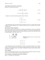
If
f(t)
is
defined outside
the

specified
interval
by a
periodic extension
of
period
27,
and if
f(t)
and
its
first
derivative
are
piecewise continuous, then
the
series
converges
to
/(O
if
f
is a
point
of
con-
tinuity,
or to
l/2
[f(t+)

+
/(*-)]
if t is a
point
of
discontinuity.
Note
that
while
the
Fourier
series
in
general
is
infinite,
the
notion
of
bandwidth
can be
used
to
reduce
the
number
of
terms required
for
a

reasonable approximation.
27.6 STATE-VARIABLE
METHODS
State-variable
methods
use the
vector
state
and
output equations introduced
in
Section
27.4
for
analysis
of
dynamic
systems
directly
in the
time
domain.
These
methods
have
several
advantages
over
transform
methods.

First,
state-variable
methods
are
particularly
advantageous
for the
study
of
multivariable
(multiple
input/multiple
output) systems. Second,
state-variable
methods
are
more
nat-
urally
extended
for the
study
of
linear
time-varying
and
nonlinear systems.
Finally,
state-variable
methods

are
readily
adapted
to
computer simulation
studies.
27.6.1
Solution
of the
State
Equation
Consider
the
vector equation
of
state
for a fixed
linear
system:
x(t)
=
Ax(i)
+
Bu(t)
The
solution
to
this
system
is

Revised
from William
J.
Palm
III,
Modeling,
Analysis
and
Control
of
Dynamic
Systems, Wiley, 1983,
by
permission
of the
publisher.
Mechanical
Engineers'Handbook,
2nd
ed., Edited
by
Myer
Kutz.
ISBN
0-471-13007-9
©
1998 John Wiley
&
Sons, Inc.
867

28.1
INTRODUCTION
868
28.2
CONTROL SYSTEM
STRUCTURE
869
28.2.1
A
Standard Diagram
870
28.2.2
Transfer Functions
870
28.2.3
System-Type
Number
and
Error
Coefficients
871
28.3
TRANSDUCERS
AND
ERROR
DETECTORS
872
28.3.1
Displacement
and

Velocity
Transducers
872
28.3.2
Temperature Transducers
874
28.3.3
Flow
Transducers
874
28.3.4
Error Detectors
874
28.3.5
Dynamic
Response
of
Sensors
875
28.4
ACTUATORS
875
28.4.1
Electromechanical
Actuators
875
28.4.2
Hydraulic Actuators
876
28.4.3

Pneumatic Actuators
878
28.5
CONTROL LAWS
880
28.5.1
Proportional
Control
881
28.5.2
Integral
Control
883
28.5.3
Proportional-Plus-Integral
Control
884
28.5.4
Derivative
Control
884
28.5.5
PID
Control
885
28.6
CONTROLLER HARDWARE
886
28.6.1 Feedback Compensation
and

Controller
Design
886
28.6.2
Electronic
Controllers
886
28.6.3 Pneumatic
Controllers
887
28.6.4
Hydraulic
Controllers
887
28.7
FURTHER
CRITERIA
FOR
GAIN
SELECTION
887
28.7.1 Performance
Indices
889
28.7.2
Optimal Control Methods
891
28.7.3
The
Ziegler-Nichols

Rules
891
28.7.4
Nonlinearities
and
Controller
Performance
892
28.7.5
Reset
Windup
893
28.8
COMPENSATION
AND
ALTERNATIVE
CONTROL
STRUCTURES
893
28.8.1
Series
Compensation
893
28.8.2
Feedback
Compensation
and
Cascade Control
893
28.8.3 Feedforward

Compensation
894
28.8.4
State-
Variable
Feedback
895
28.8.5
Pseudoderivative
Feedback
896
28.9
GRAPHICAL DESIGN
METHODS
896
28.9.1
The
Nyquist
Stability
Theorem
896
28.9.2
Systems
with
Dead-Time
Elements
898
28.9.3
Open-Loop
Design

for
PID
Control
898
28.9.4
Design with
the
Root
Locus
899
28.10
PRINCIPLES
OF
DIGITAL
CONTROL
901
28.10.1
Digital
Controller
Structure
902
28.10.2
Digital
Forms
of PID
Control
902
28.11
UNIQUELY
DIGITAL

ALGORITHMS
903
28.
1 1
.
1
Digital
Feedforward
Compensation
904
28.11.2
Control Design
in the
z-Plane
904
28.
1 1
.3
Direct
Design
of
Digital
Algorithms
908
CHAPTER
28
BASIC
CONTROL
SYSTEMS
DESIGN

William
J.
Palm
III
Mechanical
Engineering
Department
University
of
Rhode
Island
Kingston,
Rhode
Island
28.1
INTRODUCTION
The
purpose
of a
control system
is to
produce
a
desired
output.
This output
is
usually
specified
by

the
command
input,
and is
often
a
function
of
time.
For
simple
applications
in
well-structured
situ-
ations,
sequencing devices
like
timers
can be
used
as the
control system.
But
most
systems
are not
that
easy
to

control,
and the
controller
must have
the
capability
of
reacting
to
disturbances, changes
in
its
environment,
and new
input
commands.
The key
element
that
allows
a
control system
to do
this
is
feedback, which
is the
process
by
which

a
system's output
is
used
to
influence
its
behavior.
Feedback
in the
form
of the
room-temperature
measurement
is
used
to
control
the
furnace
in a
thermostatically
controlled
heating system. Figure
28.1
shows
the
feedback loop
in the
system's block

diagram, which
is a
graphical representation
of the
system's control
structure
and
logic.
Another
commonly
found control system
is the
pressure regulator
shown
in
Fig. 28.2.
Feedback
has
several
useful properties.
A
system
whose
individual
elements
are
nonlinear
can
often
be

modeled
as a
linear
one
over
a
wider range
of
its
variables
with
the
proper
use of
feedback.
This
is
because feedback tends
to
keep
the
system near
its
reference operation condition. Systems
that
can
maintain
the
output near
its

desired value
despite
changes
in the
environment
are
said
to
have
good disturbance rejection. Often
we do not
have accurate values
for
some
system parameter,
or
these
values might change with age. Feedback
can be
used
to
minimize
the
effects
of
parameter
changes
and
uncertainties.
A

system
that
has
both good disturbance
rejection
and low
sensitivity
to
parameter
variation
is
robust.
The
application
that
resulted
in the
general understanding
of the
prop-
erties
of
feedback
is
shown
in
Fig. 28.3.
The
electronic
amplifier

gain
A is
large,
but we are
uncertain
of
its
exact value.
We use the
resistors
Rl
and
R2
to
create
a
feedback loop around
the
amplifier,
and
pick
Rl
and
R2
to
create
a
feedback loop around
the
amplifier,

and
pick
Rl
and
R2
so
that
AR2/Rl
»
1.
Then
the
input-output
relation
becomes
e0
«
R^e^R^^
which
is
independent
of A as
long
as
A
remains
large.
If
Rl
and

R2
are
known
accurately, then
the
system gain
is now
reliable.
Figure
28.4
shows
the
block diagram
of a
closed-loop system, which
is a
system with feedback.
An
open-loop system, such
as a
timer,
has no
feedback. Figure 28.4
serves
as a
focus
for
outlining
the
prerequisites

for
this
chapter.
The
reader should
be
familiar with
the
transfer-function
concept
based
on the
Laplace transform,
the
pulse-transfer function based
on the
z-transform,
for
digital
control,
and the
differential
equation modeling techniques needed
to
obtain them.
It is
also
necessary
to
understand block-diagram algebra,

characteristic
roots,
the final-value
theorem,
and
their
use in
evaluating
system response
for
common
inputs
like
the
step
function. Also required
are
stability
analysis
techniques such
as the
Routh
criterion,
and
transient
performance
specifications,
such
as the
damping

ratio
£,
natural
frequency
a)n,
dominant time constant
r,
maximum
overshoot,
settling
time,
and
bandwidth.
The
above material
is
reviewed
in the
previous chapter. Treatment
in
depth
is
given
in
Refs.
1, 2, and 3.
Fig.
28.1 Block diagram
of the
thermostat

system
for
temperature
control.1
28.12
HARDWARE
AND
SOFTWARE
FOR
DIGITAL
CONTROL
909
28.12.1
Digital
Control
Hardware
909
28.12.2
Software
for
Digital
Control
911
28.13
FUTURE TRENDS
IN
CONTROL
SYSTEMS
912
28.13.1

Fuzzy
Logic Control
913
28.13.2
Neural
Networks
914
28.13.3
Nonlinear Control
914
28.13.4
Adaptive Control
914
28.13.5 Optimal Control
914
Fig.
28.2
Pressure
regulator:
(a)
cutaway
view;
(b)
block
diagram.1
28.2
CONTROL SYSTEM STRUCTURE
The
electromechanical position control
system

shown
in
Fig.
28.5
illustrates
the
structure
of a
typical
control system.
A
load with
an
inertia
/ is to be
positioned
at
some
desired angle
6r.
A dc
motor
is
provided
for
this
purpose.
The
system
contains viscous

damping,
and a
disturbance torque
Td
acts
on the
load,
in
addition
to the
motor
torque
T.
Because
of the
disturbance,
the
angular position
6 of
the
load
will
not
necessarily equal
the
desired value
6r.
For
this
reason,

a
potentiometer,
or
some
other sensor such
as an
encoder,
is
used
to
measure
the
displacement
6. The
potentiometer voltage
representing
the
controlled position
0
is
compared
to the
voltage generated
by the
command
poten-
tiometer.
This
device enables
the

operator
to
dial
in the
desired angle
dr.
The
amplifier sees
the
difference
e
between
the two
potentiometer voltages.
The
basic function
of the
amplifier
is to
increase
the
small error voltage
e up to the
voltage
level
required
by the
motor
and to
supply

enough
current
required
by the
motor
to
drive
the
load.
In
addition,
the
amplifier
may
shape
the
voltage signal
in
certain
ways
to
improve
the
performance
of the
system.
The
control
system
is

seen
to
provide
two
basic functions:
(1) to
respond
to a
command
input
that
specifies
a new
desired value
for the
controlled variable,
and (2) to
keep
the
controlled variable
near
the
desired value
in
spite
of
disturbances.
The
presence
of the

feedback
loop
is
vital
to
both
Fig.
28.3
A
closed-loop
system.
Fig. 28.4
Feedback
compensation
of an
amplifier.
functions.
A
block
diagram
of
this
system
is
shown
in
Fig. 28.6.
The
power
supplies required

for
the
potentiometers
and the
amplifier
are not
shown
in
block
diagrams
of
control
system
logic
because
they
do not
contribute
to the
control logic.
28.2.1
A
Standard
Diagram
The
electromechanical positioning
system
fits the
general structure
of a

control
system
(Fig.
28.7).
This
figure
also gives
some
standard
terminology.
Not
all
systems
can be
forced into
this
format,
but
it
serves
as a
reference
for
discussion.
The
controller
is
generally thought
of as a
logic

element
that
compares
the
command
with
the
measurement
of the
output,
and
decides
what
should
be
done.
The
input
and
feedback
elements
are
transducers
for
converting
one
type
of
signal into another type.
This

allows
the
error detector directly
to
compare
two
signals
of the
same
type (e.g.,
two
voltages).
Not all
functions
show
up as
separate
physical
elements.
The
error detector
in
Fig. 28.5
is
simply
the
input terminals
of the
amplifier.
The

control logic elements
produce
the
control signal,
which
is
sent
to the final
control elements.
These
are the
devices
that
develop
enough
torque, pressure, heat,
and so on to
influence
the
elements
under
control.
Thus,
the final
control
elements
are the
"muscle"
of the
system,

while
the
control
logic
elements
are the
"brain."
Here
we are
primarily
concerned
with
the
design
of the
logic
to be
used
by
this
brain.
The
object
to be
controlled
is the
plant.
The
manipulated
variable

is
generated
by the final
control
elements
for
this
purpose.
The
disturbance input also acts
on the
plant.
This
is an
input over
which
the
designer
has no
influence,
and
perhaps
for
which
little
information
is
available
as to the
magnitude,

functional
form,
or
time
of
occurrence.
The
disturbance
can be a
random
input,
such
as
wind
gust
on a
radar antenna,
or
deterministic,
such
as
Coulomb
friction effects.
In the
latter
case,
we can
include
the
friction

force
in the
system
model
by
using
a
nominal
value
for the
coefficient
of
friction.
The
disturbance input
would
then
be the
deviation
of the
friction force
from
this
estimated value
and
would
represent
the
uncertainty
in our

estimate.
Several control
system
classifications
can be
made
with reference
to
Fig. 28.7.
A
regulator
is a
control
system
in
which
the
controlled variable
is to be
kept constant
in
spite
of
disturbances.
The
command
input
for a
regulator
is its set

point.
A
follow-up
system
is
supposed
to
keep
the
control
variable
near
a
command
value
that
is
changing
with time.
An
example
of a
follow-up
system
is a
machine
tool
in
which
a

cutting
head
must
trace
a
specific path
in
order
to
shape
the
product properly.
This
is
also
an
example
of a
servomechanism,
which
is a
control
system
whose
controlled variable
is
a
mechanical
position, velocity,
or

acceleration.
A
thermostat
system
is not a
servomechanism,
but
a
process-control
system,
where
the
controlled variable describes
a
thermodynamic
process. Typically,
such variables
are
temperature, pressure,
flow
rate, liquid
level,
chemical
concentration,
and so on.
28.2.2
Transfer
Functions
A
transfer function

is
defined
for
each
input-output pair
of the
system.
A
specific transfer function
is
found
by
setting
all
other inputs
to
zero
and
reducing
the
block
diagram.
The
primary
or
command
transfer
function
for
Fig. 28.7

is
Fig. 28.5 Position-control
system
using
a dc
motor.1
Fig.
28.6
Block diagram
of the
position-control
system
shown
in
Fig.
28.5.1
0£)
=
A(s)Ga(s)Gm(s)Gp(S)
V(s)
1 +
Ga(s)Gm(s)Gp(s)H(S)
'
}
The
disturbance
transfer
function
is
C(s)

=
~Q(s)Gp(s)
D(s)
1 +
Ga(s)Gm(s)Gp(s)H(s)
V
'
;
The
transfer
functions
of a
given
system
all
have
the
same
denominator.
28.2.3
System-Type Number
and
Error Coefficients
The
error
signal
in
Fig.
28.4
is

related
to the
input
as
E(s)
= *
R(s)
(28.3)
1
+
G(s)H(s)
If
the final
value
theorem
can be
applied,
the
steady-state
error
is
Elements
Signals
A(s)
Input elements
B(s)
Feedback
signal
Ga(s)
Control

logic
elements
C(s)
Controlled
variable
or
output
Gm(s)
Final control elements
D(s)
Disturbance
input
Gp(s)
Plant elements
E(s)
Error
or
actuating
signal
H(s)
Feedback
elements
F(s)
Control
signal
Q(s)
Disturbance elements
M(s)
Manipulated
variable

R(s)
Reference input
V(s)
Command
input
Fig.
28.7
Terminology
and
basic
structure
of a
feedback-control
system.1
' Sfr^fe
(28-4)
The
static
error coefficient
ct
is
defined
as
c,
=
lim
slG(s}H(s}
(28.5)
s-»0
A

system
is of
type
n if
G(s)H(s)
can be
written
as
snF(s).
Table
28.1
relates
the
steady-state
error
to
the
system
type
for
three
common
inputs,
and can be
used
to
design
systems
for
minimum

error.
The
higher
the
system
type,
the
better
the
system
is
able
to
follow
a
rapidly
changing
input.
But
higher-type
systems
are
more
difficult
to
stabilize,
so a
compromise
must
be

made
in the
design.
The
coefficients
c0,
cl9
and
c2
are
called
the
position, velocity,
and
acceleration error coefficients.
28.3
TRANSDUCERS
AND
ERROR
DETECTORS
The
control
system
structure
shown
in
Fig.
28.7
indicates
a

need
for
physical devices
to
perform
several
types
of
functions.
Here
we
present
a
brief
overview
of
some
available transducers
and
error
detectors.
Actuators
and
devices used
to
implement
the
control logic
are
discussed

in
Sections 28.4
and
28.5.
28.3.1
Displacement
and
Velocity
Transducers
A
transducer
is a
device
that
converts
one
type
of
signal into another type.
An
example
is the
potentiometer,
which
converts
displacement
into voltage,
as in
Fig. 28.8.
In

addition
to
this
conver-
sion,
the
transducer
can be
used
to
make
measurements.
In
such
applications,
the
term
sensor
is
more
appropriate.
Displacement
can
also
be
measured
electrically with
a
linear variable differential trans-
former

(LVDT)
or a
synchro.
An
LVDT
measures
the
linear displacement
of a
movable
magnetic
core through
a
primary
winding
and two
secondary
windings
(Fig.
28.9).
An ac
voltage
is
applied
to
the
primary.
The
secondaries
are

connected
together
and
also
to a
detector
that
measures
the
voltage
and
phase
difference.
A
phase
difference
of 0°
corresponds
to a
positive core displacement,
while 180° indicates
a
negative
displacement.
The
amount
of
displacement
is
indicated

by the am-
plitude
of the ac
voltage
in the
secondary.
The
detector converts
this
information into
a dc
voltage
e0,
such
that
e0
=
Kx.
The
LVDT
is
sensitive
to
small displacements.
Two of
them
can be
wired
together
to

form
an
error detector.
A
synchro
is a
rotary differential transformer, with angular displacement
as
either
the
input
or
output.
They
are
often
used
in
paris
(a
transmitter
and a
receiver)
where
a
remote
indication
of
angular displacement
is

needed.
When
a
transmitter
is
used
with
a
synchro
control transformer,
two
angular displacements
can be
measured
and
compared
(Fig.
28.10).
The
output voltage
e0
is
approx-
imately linear with angular difference within
±70°,
so
that
e0
=
^(^

-
02).
Displacement
measurements
can be
used
to
obtain forces
and
accelerations.
For
example,
the
displacement
of a
calibrated spring indicates
the
applied force.
The
accelerometer
is
another
example.
Still
another
is the
strain
gage
used
for

force
measurement.
It is
based
on the
fact
that
the
resistance
of a fine
wire
changes
as it is
stretched.
The
change
in
resistance
is
detected
by a
circuit
that
can be
calibrated
to
indicate
the
applied force.
Sensors

utilizing piezoelectric
elements
are
also available.
Velocity
measurements
in
control
systems
are
most
commonly
obtained with
a
tachometer.
This
.
is
essentially
a dc
generator (the reverse
of a dc
motor).
The
input
is
mechanical
(a
velocity).
The

output
is a
generated voltage proportional
to the
velocity. Translational velocity
can be
measured
by
converting
it to
angular velocity with gears,
for
example.
Tachometers
using
ac
signals
are
also
available.
Table
28.1
Steady-State
Error
ess
for
Different
System-Type
Numbers
System

Type
Number
n
R(s)
0
123
Step
1/5
000
1
+
CQ
Ramp
1/s2
oo — 0 0
Q
Parabola
1/s3
oo oo — 0
Q
Fig. 28.8 Rotary
potentiometer.1
Other
velocity transducers include
a
magnetic
pickup
that
generates
a

pulse every time
a
gear
tooth
passes.
If the
number
of
gear
teeth
is
known,
a
pulse counter
and
timer
can be
used
to
compute
the
angular velocity.
This
principle
is
also
employed
in
turbine
flowmeters.

A
similar principle
is
employed
by
optical encoders,
which
are
especially
suitable
for
digital
control purposes.
These
devices
use a
rotating disk with alternating transparent
and
opaque
elements
whose
passage
is
sensed
by
light
beams
and a
photo-sensor array,
which

generates
a
binary
(on-off)
train
of
pulses.
There
are two
basic types:
the
absolute
encoder
and the
incremental encoder.
By
counting
the
number
of
pulses
in a
given time
interval,
the
incremental encoder
can
measure
the
rotational

speed
of the
disk.
By
using multiple tracks
of
elements,
the
absolute encoder
can
produce
a
binary
digit
that
indicates
the
amount
of
rotation.
Hence,
it can be
used
as a
position sensor.
Most
encoders generate
a
train
of TTL

voltage
level
pulses
for
each channel.
The
incremental
encoder output contains
two
channels
that
each
produce
N
pulses every revolution.
The
encoder
is
mechanically constructed
so
that
pulses
from
one
channel
are
shifted
relative
to the
other channel

by
a
quarter
of a
pulse width.
Thus,
each pulse
pair
can be
divided
into
four
segments
called
quadratures.
The
encoder
output consists
of 4N
quadrature
counts
per
revolution.
The
pulse
shift
also allows
the
Fig. 28.9 Linear
variable

differential
transformer
(LVDT).1
Fig.
28.10
Synchro
transmitter-control
transformer.1
direction
of
rotation
to be
determined
by
detecting
which
channel
leads
the
other.
The
encoder might
contain
a
third
channel,
known
as the
zero, index,
or

marker
channel,
that
produces
a
pulse once
per
revolution.
This
is
used
for
initialization.
The
gain
of
such
an
incremental encoder
is
4NI2ir.
Thus,
an
encoder with
1000
pulses
per
channel
per
revolution

has a
gain
of 636
counts
per
radian.
If an
absolute encoder produces
a
binary
signal
with
n
bits,
the
maximum
number
of
positions
it can
represent
is
2n,
and its
gain
is
2"/27r.
Thus,
a
16-bit

absolute encoder
has a
gain
of
216/27r
=
10,435
counts
per
radian.
28.3.2
Temperature
Transducers
When
two
wires
of
dissimilar
metals
are
joined together,
a
voltage
is
generated
if the
junctions
are
at
different

temperatures.
If the
reference junction
is
kept
at a fixed,
known
temperature,
the
ther-
mocouple
can be
calibrated
to
indicate
the
temperature
at the
other junction
in
terms
of the
voltage
v,
Electrical
resistance changes with temperature. Platinum gives
a
linear
relation
between

resistance
and
temperature, while nickel
is
less
expensive
and
gives
a
large
resistance change
for a
given
temperature change.
Seminconductors
designed with
this
property
are
called
thermistors. Different
metals
expand
at
different
rates
when
the
temperature
is

increased. This
fact
is
used
in the
bimetallic
strip
transducer found
in
most
home
thermostats.
Two
dissimilar metals
are
bonded
together
to
form
the
strip.
As the
temperature
rises,
the
strip
curls,
breaking contact
and
shutting

off the
furnace.
The
temperature
gap can be
adjusted
by
changing
the
distance between
the
contacts.
The
motion
also
moves
a
pointer
on the
temperature
scale
of the
thermostat. Finally,
the
pressure
of a fluid
inside
a
bulb
will

change
as its
temperature changes.
If the
bulb
fluid is
air,
the
device
is
suitable
for use in
pneumatic temperature
controllers.
28.3.3
Flow
Transducers
A flow
rate
q can be
measured
by
introducing
a flow
restriction,
such
as an
orifice
plate,
and

mea-
suring
the
pressure drop
Ap
across
the
restriction.
The
relation
is
Ap
=
Rq2,
where
R can be
found
from
calibration
of the
device.
The
pressure drop
can be
sensed
by
converting
it
into
the

motion
of
a
diaphragm. Figure
28.11
illustrates
a
related
technique.
The
Venturi-type
flowmeter
measures
the
static
pressures
in the
constricted
and
unconstricted
flow
regions. Bernoulli's
principle
relates
the
pressure
difference
to the flow
rate.
This pressure difference produces

the
diaphragm displacement.
Other types
of flowmeters are
available,
such
as
turbine meters.
28.3.4
Error
Detectors
The
error
detector
is
simply
a
device
for finding the
difference
between
two
signals.
This function
is
sometimes
an
integral
feature
of

sensors, such
as
with
the
synchro transmitter-transformer com-
bination.
This concept
is
used with
the
diaphragm element
shown
in
Fig.
28.11.
A
detector
for
voltage
difference
can be
obtained,
as
with
the
position-control system
shown
in
Fig.
28.5.

An
amplifier
intended
for
this
purpose
is a
differential
amplifier.
Its
output
is
proportional
to the
difference between
the
two
inputs.
In
order
to
detect
differences
in
other types
of
signals,
such
as
temperature, they

are
usually
converted
to a
displacement
or
pressure.
One of the
detectors mentioned previously
can
then
be
used.
Fig.
28.11
Venturi-type
flowmeter.
The
diaphragm displacement indicates
the
flow
rate.1
28.3.5
Dynamic
Response
of
Sensors
The
usual transducer
and

detector
models
are
static
models,
and as
such imply
that
the
components
respond instantaneously
to the
variable being sensed.
Of
course,
any
real
component
has a
dynamic
response
of
some
sort,
and
this
response time
must
be
considered

in
relation
to the
controlled process
when
a
sensor
is
selected.
If the
controlled process
has a
time constant
at
least
10
times greater than
that
of the
sensor,
we
often
would
be
justified
in
using
a
static
sensor

model.
28.4
ACTUATORS
An
actuator
is the final
control element
that
operates
on the
low-level control signal
to
produce
a
signal
containing
enough
power
to
drive
the
plant
for the
intended purpose.
The
armature-controlled
dc
motor,
the
hydraulic servomotor,

and the
pneumatic
diaphragm
and
piston
are
common
examples
of
actuators.
28.4.1
Electromechanical
Actuators
Figure
28.12
shows
an
electromechanical system consisting
of an
armature-controlled
dc
motor
driv-
ing
a
load
inertia.
The
rotating armature consists
of a

wire conductor
wrapped
around
an
iron core.
Fig.
28.12
Armature-controlled
dc
motor
with
a
load,
and the
system's
block
diagram,1
This
winding
has an
inductance
L. The
resistance
R
represents
the
lumped
value
of the
armature

resistance
and any
external resistance deliberately introduced
to
change
the
motor's
behavior.
The
armature
is
surrounded
by a
magnetic
field. The
reaction
of
this
field
with
the
armature
current
produces
a
torque
that
causes
the
armature

to
rotate.
If the
armature
voltage
v is
used
to
control
the
motor,
the
motor
is
said
to be
armature-controlled.
In
this
case,
the field is
produced
by an
electro-
magnet
supplied with
a
constant voltage
or by a
permanent

magnet.
This
motor
type
produces
a
torque
T
that
is
proportional
to the
armature
current
ia:
T =
KTia
(28.6)
The
torque constant
KT
depends
on the
strength
of the
field
and
other
details
of the

motor's
construc-
tion.
The
motion
of a
current-carrying
conductor
in a field
produces
a
voltage
in the
conductor
that
opposes
the
current.
This
voltage
is
called
the
back
emf
(electromotive
force).
Its
magnitude
is

proportional
to the
speed
and is
given
by
eb
=
Kea>
(28.7)
The
transfer function
for the
armature-controlled
dc
motor
is
OW
=
KT
V(s)
LIs2
+
(RI
+
cL)s
+ cR +
KeKT
^
'

)
Another
motor
configuration
is the field-controlled dc
motor.
In
this
case,
the
armature
current
is
kept constant
and the field
voltage
v is
used
to
control
the
motor.
The
transfer function
is
Q(')
_
KT
(2o9}
V(s)

(Ls +
R)(Is
+ c)
where
R and L are the
resistance
and
inductance
of the
field
circuit,
and
KT
is the
torque constant.
No
back
emf
exists
in
this
motor
to act as a
self-braking
mechanism.
Two-phase
ac
motors
can be
used

to
provide
a
low-power,
variable-speed actuator.
This
motor
type
can
accept
the ac
signals directly
from
LVDTs
and
synchros
without
demodulation.
However,
it
is
difficult
to
design
ac
amplifier circuitry
to do
other than proportional action.
For
this

reason,
the
ac
motor
is not
found
in
control
systems
as
often
as dc
motors.
The
transfer function
for
this
type
is
of the
form
of Eq.
(28.9).
An
actuator especially suitable
for
digital
systems
is the
stepper motor,

a
special
dc
motor
that
takes
a
train
of
electrical
input pulses
and
converts
each
pulse into
an
angular displacement
of a
fixed
amount.
Motors
are
available with resolutions ranging
from
about
4
steps
per
revolution
to

more
than
800
steps
per
revolution.
For 36
steps
per
revolution,
the
motor
will rotate
by 10° for
each
pulse received.
When
not
being pulsed,
the
motors
lock
in
place.
Thus,
they
are
excellent
for
precise

positioning applications,
such
as
required with printers
and
computer
tape drives.
A
disadvantage
is
that
they
are
low-torque
devices.
If the
input pulse
frequency
is not
near
the
resonant
frequency
of
the
motor,
we can
take
the
output rotation

to be
directly related
to the
number
of
input pulses
and
use
that
description
as the
motor
model.
28.4.2
Hydraulic
Actuators
Machine
tools
are one
application
of the
hydraulic
system
shown
in
Fig.
28.13.
The
applied force
/

is
supplied
by the
servomotor.
The
mass
m
represents
that
of a
cutting tool
and the
power
piston,
while
k
represents
the
combined
effects
of the
elasticity
naturally present
in the
structure
and
that
introduced
by the
designer

to
achieve proper
performance.
A
similar statement applies
to the
damping
c.
The
valve displacement
z is
generated
by
another control
system
in
order
to
move
the
tool through
its
prescribed
motion.
The
spool valve
shown
in
Fig.
28.13

had two
lands.
If the
width
of the
land
is
greater than
the
port width,
the
valve
is
said
to be
overlapped.
In
this
case,
a
dead
zone
exists
in
which
a
slight
change
in the
displacement

z
produces
no
power
piston
motion.
Such
dead
zones
create
control
difficulties
and are
avoided
by
designing
the
valve
to be
underlapped
(the land
width
is
less
the
port
width).
For
such
valves there will

be a
small
flow
opening
even
when
the
valve
is in
the
neutral position
at z = 0.
This
gives
it a
higher
sensitivity
than
an
overlapped valve.
The
variables
z and
A/?
=
p2
-
pl
determine
the

volume
flow
rate,
as
q
=
/feAp)
For the
reference equilibrium condition
(z = 0,
Ap
= 0, q — 0), a
linearization gives
q
=
Clz-
C2A/7
(28.10)
Modeled
as f
rictionless
Fig.
28.13
Hydraulic
servomotor
with
a
load.1
The
linearization

constants
are
available
from
theoretical
and
experimental
results.4
The
transfer
function
for the
system
is1'2
™-H-C*n_(c£+\
C*
(28-U>
—-
s2
+
(-—
+
A)s
+
—-
A \ A
/
A
The
development

of the
steam engine
led to the
requirement
for a
speed-control
device
to
maintain
constant
speed
in the
presence
of
changes
in
load torque
or
steam pressure.
In
1788, James Watt
of
Glasgow
developed
his
now-famous
flyball
governor
for
this

purpose (Fig.
28.14).
Watt took
the
principle
of
sensing speed with
the
centrifugal
pendulum
of
Thomas
Mead
and
used
it
in a
feedback
loop
on a
steam engine.
As the
motor
speed
increases,
the
flyballs
move
outward
and

pull
the
slider
Fig.
28.14
James
Watt's
flyball
governor
for
speed
control
of a
steam
engine.1
Fig.
28.15
Electrohydraulic
system
for
translation.1
upward.
The
upward
motion
of the
slider
closes
the
steam

valve, thus causing
the
engine
to
slow
down.
If the
engine speed
is too
slow,
the
spring force
overcomes
that
due to the flyballs, and the
slider
moves
down
to
open
the
steam
valve.
The
desired speed
can be set by
moving
the
plate
to

change
the
compression
in the
spring.
The
principle
of the flyball
governor
is
still
used
for
speed-
control
applications. Typically,
the
pilot
valve
of a
hydraulic
servomotor
is
connected
to the
slider
to
provide
the
high forces required

to
move
large supply valves.
Many
hydraulic servomotors
use
multistage valves
to
obtain
finer
control
and
higher forces.
A
two-stage valve
has a
slave value, similar
to the
pilot
valve,
but
situated
between
the
pilot
valve
and
the
power
piston.

Rotational
motion
can be
obtained with
a
hydraulic motor,
which
is, in
principle,
a
pump
acting
in
reverse (fluid input
and
mechanical rotation output).
Such
motors
can
achieve higher torque
levels
than
electric
motors.
A
hydraulic
pump
driving
a
hydraulic

motor
constitutes
a
hydraulic transmission.
A
popular actuator choice
is the
electrohydraulic system,
which
uses
an
electric
actuator
to
control
a
hydraulic
servomotor
or
transmission
by
moving
the
pilot
valve
or the
swash-plate angle
of the
pump.
Such

systems
combine
the
power
of
hydraulics with
the
advantages
of
electrical
systems.
Figure
28.15
shows
a
hydraulic
motor
whose
pilot
valve
motion
is
caused
by an
armature-controlled
dc
motor.
The
transfer function
between

the
motor
voltage
and the
piston displacement
is
X(s)
KlK2Cl
W)
=
As^rs
+ 1)
(28'12)
If
the
rotational
inertia
of the
electric
motor
is
small, then
r
~
0.
28.4.3
Pneumatic
Actuators
Pneumatic
actuators

are
commonly
used because they
are
simple
to
maintain
and use a
readily
available
working
medium.
Compressed
air
supplies with
the
pressures required
are
commonly
avail-
able
in
factories
and
laboratories.
No flammable fluids or
electrical
sparks
are
present,

so
these devices
are
considered
the
safest
to use
with chemical processes. Their
power
output
is
less
than
that
of
hydraulic systems,
but
greater than
that
of
electric
motors.
A
device
for
converting pneumatic pressure into displacement
is the
bellows
shown
in

Fig.
28.16.
The
transfer function
for a
linearized
model
of the
bellows
is of the
form
^
=
-*-
(28.13)
P(s)
rs + 1
where
x and p are
deviations
of the
bellows displacement
and
input pressure
from
nominal
values.
In
many
control applications,

a
device
is
needed
to
convert small displacements
into
relatively
large
pressure changes.
The
nozzle-flapper serves
this
purpose (Fig.
28.17a).
The
input displacement
y
moves
the flapper,
with
little
effort required. This changes
the
opening
at the
nozzle
orifice.
For a
Fig. 28.16

Pneumatic
bellows.1
Fig. 28.17
Pneumatic
nozzle-flapper
amplifier
and
its
characteristic
curve.1
large
enough
opening,
the
nozzle
back
pressure
is
approximately
the
same
as
atmospheric
pressure
pa.
At the
other
extreme
position with
the flapper

completely blocking
the
orifice,
the
back
pressure
equals
the
supply pressure
ps.
This variation
is
shown
in
Fig.
28.176.
Typical
supply
pressures
are
between
30 and 100
psia.
The
orifice
diameter
is
approximately 0.01
in.
Flapper displacement

is
usually less than
one
orifice
diameter.
The
nozzle-flapper
is
operated
in the
linear portion
of the
back
pressure curve.
The
linearized
back
pressure relation
is
p
=
-Kjx
(28.14)
where
-Kf
is the
slope
of the
curve
and is a

very large
number.
From
the
geometry
of
similar
triangles,
we
have
P j±y
(2,15)
In
its
operating region,
the
nozzle-flapper's
back
pressure
is
well
below
the
supply pressure.
The
output pressure
from
a
pneumatic
device

can be
used
to
drive
a final
control element
like
the
pneumatic
actuating valve
shown
in
Fig.
28.18.
The
pneumatic
pressure
acts
on the
upper side
of the
diaphragm
and is
opposed
by the
return spring.
Formerly,
many
control systems
utilized

pneumatic
devices
to
implement
the
control
law in
analog
form.
Although
the
overall,
or
higher-level, control algorithm
is now
usually
implemented
in
digital
form,
pneumatic
devices
are
still
frequently used
for final
control corrections
at the
actuator level,
Fig. 28.18

Pneumatic
flow-control
valve.1
where
the
control action
must
eventually
be
supplied
by a
mechanical
device.
An
example
of
this
is
the
electro-pneumatic valve positioner used
in
Valtek valves,
and
illustrated
in
Fig.
28.19.
The
heart
of the

unit
is a
pilot valve capsule
that
moves
up and
down
according
to the
pressure difference
across
its two
supporting
diaphragms.
The
capsule
has a
plunger
at its top and at its
bottom.
Each
plunger
has an
exhaust seat
at one end and a
supply
seat
at the
other.
When

the
capsule
is in its
equilibrium position,
no air is
supplied
to or
exhausted
from
the
valve cylinder,
so the
valve does
not
move.
The
process controller
commands
a
change
in the
valve
stem
position
by
sending
the
4-20
ma
dc

input signal
to the
positioner. Increasing
this
signal causes
the
electromagnetic actuator
to
rotate
the
lever counterclockwise about
the
pivot. This increases
the air gap
between
the
nozzle
and flapper.
This decreases
the
back
pressure
on top of the
upper
diaphragm
and
causes
the
capsule
to

move
up.
This
motion
lifts
the
upper plunger
from
its
supply
seat
and
allows
the
supply
air to flow to the
bottom
of the
valve cylinder.
The
lower
plunger's exhaust seat
is
uncovered,
thus decreasing
the air
pressure
on top of the
valve piston,
and the

valve
stem
moves
upward.
This
motion
causes
the
lever
arm to
rotate, increasing
the
tension
in the
feedback
spring
and
decreasing
the
nozzle-flapper gap.
The
valve continues
to
move
upward
until
the
tension
in the
feedback

spring counteracts
the
force
produced
by the
electromagnetic actuator, thus returning
the
capsule
to its
equilibrium position.
A
decrease
in the dc
input signal causes
the
opposite actions
to
occur,
and the
valve
moves
downward.
28.5
CONTROL LAWS
The
control logic elements
are
designed
to act on the
error signal

to
produce
the
control signal.
The
algorithm
that
is
used
for
this
purpose
is
called
the
control law,
the
control action,
or the
control
algorithm.
A
nonzero
error signal
results
from
either
a
change
in

command
or a
disturbance.
The
general function
of the
controller
is to
keep
the
controlled variable near
its
desired value
when
these
occur.
More
specifically,
the
control objectives
might
be
stated
as
follows:
1.
Minimize
the
steady-state error.
2.

Minimize
the
settling
time.
3.
Achieve
other transient specifications, such
as
minimizing
the
overshoot.
Fig.
28.19
An
electro-pneumatic valve positioner.
In
practice,
the
design specifications
for a
controller
are
more
detailed.
For
example,
the
bandwidth
might
also

be
specified along with
a
safety
margin
for
stability.
We
never
know
the
numerical values
of
the
system's
parameters with true certainty,
and
some
controller designs
can be
more
sensitive
to
such parameter uncertainties than other designs.
So a
parameter
sensitivity
specification
might
also

be
included.
The
following control laws
form
the
basis
of
most
control systems.
28.5.1
Proportional
Control
Two-position control
is the
most
familiar type, perhaps
because
of
its
use in
home
thermostats.
The
control
output takes
on one of two
values.
With
the

on-off
controller,
the
controller output
is
either
on or off
(e.g.,
fully
open
or
fully
closed).
Two-position
control
is
acceptable
for
many
applications
in
which
the
requirements
are not too
severe.
However,
many
situations require
finer

control.
Consider
a
liquid-level
system
in
which
the
input
flowrate is
controlled
by a
valve.
We
might
try
setting
the
control valve
manually
to
achieve
a flow
rate
that
balances
the
system
at the
desired

level.
We
might
then
added
a
controller
that
adjusts
this
setting
in
proportion
to the
deviation
of the
level
from
the
desired value.
This
is
proportional control,
the
algorithm
in
which
the
change
in the

control
signal
is
proportional
to the
error.
Block
diagrams
for
controllers
are
often
drawn
in
terms
of the
deviations
from
a
zero-error equilibrium condition.
Applying
this
convention
to the
general termi-
nology
of
Fig.
28.6,
we see

that
proportional control
is
described
by
F(s)
=
KPE(s)
where
F(s)
is the
deviation
in the
control signal
and
KP
is the
proportional gain.
If the
total
valve
displacement
is
y(t)
and the
manually
created displacement
is
jc,
then

y(f)
=
Kpe(t)
+ x
The
percent
change
in
error
needed
to
move
the
valve
full
scale
is the
proportional
band.
It is
related
to
the
gain
as
K
10°
p
band%
The

zero-error valve displacement
x is the
manual
reset.
Proportional
Control
of a
First-Order
System
To
investigate
the
behavior
of
proportional control, consider
the
speed-control
system
shown
in
Fig.
28.20;
it is
identical
to the
position controller
shown
in
Fig.
28.6,

except
that
a
tachometer replaces
the
feedback
potentiometer.
We can
combine
the
amplifier gains into
one,
denoted
KP.
The
system
is
thus seen
to
have proportional control.
We
assume
the
motor
is
field-controlled
and has a
negligible
electrical
time constant.

The
disturbance
is a
torque
Td,
for
example,
resulting
from
friction.
Choose
the
reference equilibrium condition
to be
Td
= T = 0 and
ct>r
=
w
= 0. The
block
diagram
is
shown
in
Fig.
28.21.
For a
meaningful
error signal

to be
generated,
Kv
and
K2
should
be
chosen
to be
equal.
With
this
simplification
the
diagram
becomes
that
shown
in
Fig.
28.22,
where
G(s)
= K —
K1KP
KTIR.
A
change
in
desired speed

can be
simulated
by a
unit step input
for
o>r.
For
£lr(s)
=1/5,
the
velocity
approaches
the
steady-state value
coss
=
Kl(c
+ K) <
1.
Thus,
the
final
value
is
less
than
the
desired value
of 1, but it
might

be
close
enough
if the
damping
c is
small.
The
time required
to
Fig.
28.20
Velocity-control
system
using
a dc
motor.1
Fig. 28.21 Block diagram
of the
velocity-control
system
of
Fig.
28.20.1
reach
this
value
is
approximately four
time

constants,
or
4r
=
4//(c
+
K}.
A
sudden
change
in
load
torque
can
also
be
modeled
by a
unit step function
Td(s)
=
l/s.
The
steady-state response
due
solely
to
the
disturbance
is —

l/(c
+
K}.
If (c +
K}
is
large,
this
error will
be
small.
The
performance
of the
proportional control
law
thus
far can be
summarized
as
follows.
For a
first-order
plant
with step function inputs:
1.
The
output never reaches
its
desired value

if
damping
is
present
(c
^
0),
although
it
can be
made
arbitrarily
close
by
choosing
the
gain
K
large
enough.
This
is
called
offset
error.
2. The
output approaches
its
final
value without oscillation.

The
time
to
reach
this
value
is
inversely
proportional
to K.
3. The
output deviation
due to the
disturbance
at
steady
state
is
inversely proportional
to the
gain
K.
This error
is
present even
in the
absence
of
damping
(c = 0).

As the
gain
K
is
increased,
the
time constant
becomes
smaller
and the
response faster.
Thus,
the
chief
disadvantage
of
proportional control
is
that
it
results
in
steady-state errors
and can
only
be
used
when
the
gain

can be
selected large
enough
to
reduce
the
effect
of the
largest expected disturbance.
Since proportional control gives zero error only
for one
load condition (the reference equilibrium),
the
operator
must
change
the
manual
reset
by
hand
(hence
the
name).
An
advantage
to
proportional
control
is

that
the
control signal responds
to the
error instantaneously
(in
theory
at
least).
It is
used
in
applications requiring rapid action. Processes with time constants
too
small
for the use of
two-
position
control
are
likely
candidates
for
proportional control.
The
results
of
this
analysis
can be

applied
to any
type
of first-order
system
(e.g., liquid-level, thermal, etc.) having
the
form
in
Fig.
28.22.
Proportional
Control
of a
Second-Order
System
Proportional control
of a
neutrally stable second-order plant
is
represented
by the
position controller
of
Fig. 28.6
if
the
amplifier transfer function
is a
constant

Ga(s)
=
Ka.
Let the
motor
transfer function
be
Gm(s)
=
KTIR,
as
before.
The
modified block
diagram
is
given
in
Fig.
28.23
with G(s)
=
K =
KlKaKT/R.
The
closed-loop
system
is
stable
if

7,
c, and K are
positive.
For no
damping
(c = 0), the
closed-loop system
is
neutrally stable.
With
no
disturbance
and a
unit step
command,
®r(s)
=
1/5,
the
steady-state output
is
coss
=
1.
The
offset
error
is
thus zero
if the

system
is
stable
(c > 0, K >
0). The
steady-state output deviation
due to a
unit step disturbance
is
—l/K.
This
deviation
can be
reduced
by
choosing
K
large.
The
transient behavior
is
indicated
by the
damping
ratio,
£
=
cl
2VlK.
For

slight
damping,
the
response
to a
step input will
be
very oscillatory
and the
overshoot large.
The
situation
is
aggravated
if the
gain
K is
made
large
to
reduce
the
deviation
due to the
disturbance.
We
conclude, therefore,
that
proportional control
of

this
type
of
second-order plant
is not a
good
choice unless
the
damping
constant
c is
large.
We
will
see
shortly
how to
improve
the
design.
Fig.
28.22
Simplified
form
of
Fig. 28.21
for
the
case
K,

=
K2.
Fig.
28.23
Position
servo.
28.5.2
Integral
Control
The
offset error
that
occurs with proportional control
is a
result
of the
system
reaching
an
equilibrium
in
which
the
control signal
no
longer
changes.
This
allows
a

constant error
to
exist.
If the
controller
is
modified
to
produce
an
increasing signal
as
long
as the
error
is
nonzero,
the
offset
might
be
eliminated.
This
is the
principle
of
integral control.
In
this
mode

the
change
in the
control signal
is
proportional
to the
integral
of the
error.
In the
terminology
of
Fig. 28.7,
this
gives
KI
F(s)
=
—E(s}
(28.16)
where
F(s)
is the
deviation
in the
control signal
and
Kj
is the

integral gain.
In the
time
domain,
the
relation
is
f(t)
=
K,
£
e(t)
dt
(28.17)
if
/(O)
=
0. In
this
form,
it can be
seen that
the
integration
cannot
continue indefinitely
because
it
would
theoretically

produce
an
infinite
value
of
f(t)
if
e(t)
does
not
change
sign.
This
implies
that
special
care
must
be
taken
to
reinitialize
a
controller that uses integral action.
Integral
Control
of a
First-Order
System
Integral

control
of the
velocity
in the
system
of
Fig.
28.20
has the
block
diagram
shown
in
Fig.
28.22,
where
G(s)
=
K/s,
K =
K^K^IR.
The
integrating action
of the
amplifier
is
physically
obtained
by the
techniques

to be
presented
in
Section 28.6,
or by the
digital
methods
presented
in
Section
28.10.
The
control
system
is
stable
if
7,
c, and K are
positive.
For a
unit step
command
input,
a)ss
= 1; so the
offset error
is
zero.
For a

unit step disturbance,
the
steady-state deviation
is
zero
if
the
system
is
stable.
Thus,
the
steady-state
performance
using integral control
is
excellent
for
this
plant
with step inputs.
The
damping
ratio
is
£
=
c/2v7JK.
For
slight

damping,
the
response will
be
oscillatory rather than exponential
as
with proportional control.
Improved
steady-state
performance
has
thus
been
obtained
at the
expense
of
degraded
transient
performance.
The
conflict
between
steady-
state
and
transient specifications
is a
common
theme

in
control
system
design.
As
long
as the
system
is
underdamped,
the
time constant
is r
=
211
c and is not
affected
by the
gain
K,
which
only influences
the
oscillation
frequency
in
this
case.
It
might

by
physically possible
to
make
K
small
enough
so
that
£
»
1, and
the
nonoscillatory
feature
of
proportional control recovered,
but
the
response
would
tend
to be
sluggish. Transient specifications
for
fast
response generally require
that
£ <
I.

The
difficulty
with using
£ < 1 is
that
r
is
fixed
by c and /. If c and / are
such
that
£ <
1,
then
r
is
large
if
/»
c.
Integral
Control
of a
Second-Order
System
Proportional control
of the
position
servomechanism
in

Fig.
28.23
gives
a
nonzero
steady-state
de-
viation
due to the
disturbance. Integral control [G(s)
=
K/s] applied
to
this
system
results
in the
command
transfer function
»(*)
_ K
ex*)
~
ft3
+
cs*
+ K
(28'18)
With
the

Routh
criterion,
we
immediately
see
that
the
system
is not
stable
because
of the
missing
s
term.
Integral control
is
useful
in
improving
steady-state
performance,
but in
general
it
does
not
improve
and may
even

degrade
transient
performance.
Improperly
applied,
it
can
produce
an
unstable
control
system.
It is
best
used
in
conjunction
with other control
modes.
28.5.3
Proportional-Plus-lntegral
Control
Integral
control raised
the
order
of the
system
by one in the
preceding

examples,
but did not
give
a
characteristic
equation with
enough
flexibility
to
achieve acceptable transient behavior.
The
instan-
taneous response
of
proportional control action
might
introduce
enough
variability
into
the
coeffi-
cients
of the
characteristic equation
to
allow both steady-state
and
transient specifications
to be

satisfied.
This
is the
basis
for
using proportional-plus-integral control
(PI
control).
The
algorithm
for
this
two-mode
control
is
Kj
F(s)
=
KPE(s}
+
—
E(s)
(28.19)
The
integral action provides
an
automatic,
not
manual,
reset

of the
controller
in the
presence
of a
disturbance.
For
this
reason,
it is
often called reset action.
The
algorithm
is
sometimes
expressed
as
F(s)
=
KP(l+^-}
E(s) (28.20)
\
1is/
where
Tl
is the
reset
time.
The
reset

time is the
time required
for the
integral action signal
to
equal
that
of the
proportional term,
if a
constant error
exists
(a
hypothetical situation).
The
reciprocal
of
reset
time
is
expressed
as
repeats
per
minute
and is the
frequency with
which
the
integral action

repeats
the
proportional correction signal.
The
proportional control gain
must
be
reduced
when
used with integral action.
The
integral
term
does
not
react instantaneously
to a
zero-error signal
but
continues
to
correct,
which
tends
to
cause
oscillations
if the
designer does
not

take
this
effect into account.
PI
Control
of a
First-Order
System
PI
action applied
to the
speed controller
of
Fig.
28.20
gives
the
diagram
shown
in
Fig.
28.21
with
G(s)
=
KP
+
Kjls.
The
gains

KP
and
Kt
are
related
to the
component
gains,
as
before.
The
system
is
stable
for
positive values
of
KP
and
Kr
For
£lr(s)
=
\ls,
a)ss
=
1,
and the
offset error
is

zero,
as
with integral action only. Similarly,
the
deviation
due to a
unit step disturbance
is
zero
at
steady
state.
The
damping
ratio
is
£
= (c +
KP)/2^/LKI.
The
presence
of
KP
allows
the
damping
ratio
to
be
selected without

fixing the
value
of the
dominant
time constant.
For
example,
if the
system
is
underdamped
(f
< 1), the time
constant
is
r
=
2/7
(c +
KP).
The
gain
KP
can be
picked
to
obtain
the
desired time constant, while
Kt

used
to
set,
the
damping
ratio.
A
similar
flexibility
exists
if
£
=
1.
Complete
description
of the
transient response requires
that
the
numerator
dynamics
present
in the
transfer
functions
be
accounted
for.1'2
PI

Control
of a
Second-Order
System
Integral
control
for the
position
servomechanism
of
Fig.
28.23
resulted
in a
third-order
system
that
is
unstable.
With
proportional action,
the
diagram
becomes
that
of
Fig.
28.22,
with
G(s)

=
KP
+
Kjls.
The
steady-state
performance
is
acceptable,
as
before,
if the
system
is
assumed
to be
stable.
This
is
true
if the
Routh
criterion
is
satisfied;
that
is, if /, c,
KP,
and
Kt

are
positive
and
cKP
—
IKt
> 0. The
difficulty
here occurs
when
the
damping
is
slight.
For
small
c, the
gain
KP
must
be
large
in
order
to
satisfy
the
last
condition,
and

this
can be
difficult
to
implement
physically.
Such
a
condition
can
also
result
in an
unsatisfactory time constant.
The
root-locus
method
of
Section
28.9
provides
the
tools
for
analyzing
this
design further.
28.5.4
Derivative
Control

Integral
action tends
to
produce
a
control signal even
after
the
error
has
vanished,
which
suggests
that
the
controller
be
made
aware
that
the
error
is
approaching zero.
One way to
accomplish
this
is
to
design

the
controller
to
react
to the
derivative
of the
error with derivative control action,
which
is
F(s)
=
KDsE(s}
(28.21)
where
KD
is the
derivative gain.
This
algorithm
is
also called rate action.
It is
used
to
damp
out
oscillations.
Since
it

depends
only
on the
error rate, derivative control should never
be
used
alone.
When
used with proportional action,
the
following
PD-control
algorithm results:
F(s)
=
(KP
+
KDs}E(s}
=
KP(l
+
TDs)E(s)
(28.22)
where
TD
is the
rate time
or
derivative time.
With

integral action included,
the
proportional-plus-
integral-plus-derivative
(PID)
control
law is
obtained.
F(s)
=
(KP
+ - +
K^\
E(s)
(28.23)
\
s
/
This
is
called
a
three-mode
controller.
PD
Control
of a
Second-Order
System
The

presence
of
integral action
reduces
steady-state error,
but
tends
to
make
the
system
less
stable.
There
are
applications
of the
position
servomechanism
in
which
a
nonzero
derivation resulting
from
the
disturbance
can be
tolerated,
but an

improvement
in
transient
response
over
the
proportional
control result
is
desired. Integral action
would
not be
required,
but
rate action
can be
added
to
improve
the
transient
response.
Application
of PD
control
to
this
system
gives
the

block
diagram
of
Fig.
28.23
with
GO) =
KP
+
K^.
The
system
is
stable
for
positive values
of
KD
and
KP.
The
presence
of
rate action
does
not
affect
the
steady-state response,
and the

steady-state results
are
identical
to
those with
P
control;
namely,
zero
offset error
and a
deviation
of
—\"lKP,
due to the
disturbance.
The
damping
ratio
is
f
= (c +
KD)/2^IKP.
For P
control,
£
=
c/2^/IKP.
Introduction
of

rate action allows
the
proportional gain
KP
to be
selected large
to
reduce
the
steady-state deviation,
while
KD
can be
used
to
achieve
an
acceptable
damping
ratio.
The
rate action also helps
to
stabilize
the
system
by
adding
damping
(if

c = 0 the
system
with
P
control
is not
stable).
The
equivalent
of
derivative action
can be
obtained
by
using
a
tachometer
to
measure
the
angular
velocity
of the
load.
The
block
diagram
is
shown
in

Fig.
28.24.
The
gain
of the
amplifier-
motor-potentiometer
combination
is
Kl,
and
K2
is the
tachometer
gain.
The
advantage
of
this
system
is
that
it
does
not
require signal differentiation,
which
is
difficult
to

implement
if
signal noise
is
present.
The
gains
i^
and
K2
can be
chosen
to
yield
the
desired
damping
ratio
and
steady-state
deviation,
as was
done
with
KP
and
Kr.
28.5.5
PID
Control

The
position
servomechanism
design with
PI
control
is not
completely
satisfactory
because
of the
difficulties
encountered
when
the
damping
c is
small.
This
problem
can be
solved
by the use of the
full
PID-control
law,
as
shown
in
Fig.

28.23
with
G(s)
=
KP
+
KpS
+
Kfls.
A
stable
system
results
if
all
gains
are
positive
and if (c +
KD)KP
-
!Kt
> 0. The
presence
of
KD
relaxes
somewhat
the
requirement

that
KP
be
large
to
achieve
stability.
The
steady-state errors
are
zero,
and the
transient
response
can be
improved
because
three
of the
coefficients
of the
char-
acteristic
equation
can be
selected.
To
make
further statements requires
the

root locus technique
presented
in
Section 28.9.
Proportional,
integral,
and
derivative actions
and
their various
combinations
are not the
only
control
laws
possible,
but
they
are the
most
common.
PID
controllers will
remain
for
some
time
the
standard against
which

any new
designs
must
compete.
The
conclusions
reached
concerning
the
performance
of the
various control
laws
are
strictly
true
only
for the
plant
model
forms
considered.
These
are the
first-order
model
without
numerator
dy-
namics

and the
second-order
model
with
a
root
at 5 = 0 and no
numerator
zeros.
The
analysis
of a
control
law for any
other linear
system
follows
the
preceding
pattern.
The
overall
system
transfer
functions
are
obtained,
and all of the
linear
system

analysis techniques
can be
applied
to
predict
the
system's
performance.
If the
performance
is
unsatisfactory,
a new
control
law is
tried
and the
process
repeated.
When
this
process
fails
to
achieve
an
acceptable design,
more
systematic
methods

of
altering
the
system's
structure
are
needed;
they
are
discussed
in
later
sections.
We
have
used
step functions
as
the
test
signals
because
they
are the
most
common
and
perhaps
represent
the

severest
test
of
system
performance.
Impulse,
ramp,
and
sinusoidal
test
signals
are
also
employed.
The
type
to use
should
be
made
clear
in the
design specifications.
Fig.
28.24
Tachometer
feedback
arrangement
to
replace

PD
control
for the
position
servo.1
28.6
CONTROLLER HARDWARE
The
control
law
must
be
implemented
by a
physical device before
the
control engineer's task
is
complete.
The
earliest
devices
were
purely kinematic
and
were
mechanical elements such
as
gears,
levers,

and
diaphragms
that
usually obtained
their
power
from
the
controlled variable.
Most
controllers
now are
analog electronic, hydraulic,
pneumatic,
or
digital
electronic devices.
We now
consider
the
analog type. Digital controllers
are
covered
starting
in
Section
28.10.
28.6.1
Feedback
Compensation

and
Controller
Design
Most
controllers
that
implement
versions
of the
PID
algorithm
are
based
on the
following feedback
principle.
Consider
the
single-loop system
shown
in
Fig.
28.1.
If the
open-loop transfer function
is
large
enough
that
\G(s)H(s)\

»
1,
the
closed-loop transfer function
is
approximately given
by
T™
=
G^
„
G^
=
_L
(2*24}
^
}
1 +
G(s)H(s)
G(s)H(s)
H(s)
V
'
The
principle
states
that
a
power
unit

G(s)
can be
used with
a
feedback element
H(s)
to
create
a
desired
transfer function
T(s).
The
power
unit
must
have
a
gain high
enough
that
\G(s)H(s)\
»
1,
and the
feedback elements
must
be
selected
so

that
H(s)
=
\IT(s).
This principle
was
used
in
Section
28.1
to
explain
the
design
of a
feedback amplifier.
28.6.2
Electronic Controllers
The
operational amplifier
(op
amp)
is a
high-gain amplifier with
a
high input
impedance.
A
diagram
of

an op amp
with feedback
and
input elements with
impedances
Tf(s)
and
Tt(s)
is
shown
in
Fig.
28.25.
An
approximate relation
is
E0(s)
=
Tf(s)
E£s)
T£s)
The
various control
modes
can be
obtained
by
proper selection
of the
impedances.

A
proportional
controller
can be
constructed with
a
multiplier,
which
uses
two
resistors,
as
shown
in
Fig.
28.26.
An
inverter
is a
multiplier
circuit
with
Rf
=
Rf.
It is
sometimes
needed because
of the
sign reversal

property
of the op
amp.
The
multiplier
circuit
can be
modified
to act as an
adder (Fig.
28.27).
PI
control
can be
implemented
with
the
circuit
of
Fig.
28.28.
Figure.
28.29
shows
a
complete
system using
op
amps
for PI

control.
The
inverter
is
needed
to
create
an
error detector.
Many
industrial
controllers
provide
the
operator with
a
choice
of
control
modes,
and the
operator
can
switch
from
one
mode
to
another
when

the
process
characteristics
or
control objectives change.
When
a
switch
occurs,
it is
necessary
to
provide
any
integrators with
the
proper
initial
voltages,
or
else
undesirable
transients
will
occur
when
the
integrator
is
switched

into
the
system.
Commercially
available con-
trollers
usually have
built-in
circuits
for
this
purpose.
In
theory,
a
differentiator
can be
created
by
interchanging
the
resistance
and
capacitance
in the
integrating
op
amp.
The
difficulty

with
this
design
is
that
no
electrical
signal
is
"pure."
Contamination
always
exists
as a
result
of
voltage spikes, ripple,
and
other transients generally categorized
as
"noise."
These
high-frequency signals have
large
slopes
compared
with
the
more
slowly varying

primary signal,
and
thus they
will
dominate
the
output
of the
differentiator.
In
practice,
this
problem
is
solved
by
filtering
out
high-frequency signals,
either
with
a
low-pass
filter
inserted
in
cascade with
the
differentiator,
or by

using
a
redesigned
differentiator
such
as the one
shown
in
Fig.
28.30.
For
the
ideal
PD
controller,
Rl
= 0. The
attenuation curve
for the
ideal
controller breaks
upward
at
a>
=
l/R2C
with
a
slope
of 20

db/decade.
The
curve
for the
practical
controller does
the
same
but
then
becomes
flat
for
a)>
(R{
+
R2)/R1R2C.
This provides
the
required limiting
effect
at
high frequencies.
PID
control
can be
implemented
by
joining
the PI and PD

controllers
in
parallel,
but
this
is
expensive because
of the
number
of op
amps
and
power
supplies required. Instead,
the
usual imple-
mentation
is
that
shown
in
Fig.
28.31.
The
circuit
limits
the
effect
of
frequencies above

co
=
II
Fig.
28.25
Operational
amplifier
(op
amp).1
Fig.
28.26
Op-amp
implementation
of
proportional
control.1
/3/^Q.
When
/^
=
0,
ideal
PID
control
results.
This
is
sometimes
called
the

noninteractive algorithm
because
the
effect
of
each
of the
three
modes
is
additive,
and
they
do not
interfere with
one
another.
The
form
given
for
Rv
+
0 is the
real
or
interactive
algorithm. This
name
results

from
the
fact
that
historically
it was
difficult
to
implement
noninteractive
PID
control with
mechanical
or
pneumatic
devices.
28.6.3
Pneumatic
Controllers
The
nozzle-flapper introduced
in
Section
28.4
is a
high-gain device
that
is
difficult
to use

without
modification.
The
gain
Kf
is
known
only imprecisely
and is
sensitive
to
changes induced
by
tem-
perature
and
other environmental factors. Also,
the
linear region over
which
Eq.
(28.14)
applies
is
very small.
However,
the
device
can be
made

useful
by
compensating
it
with
feedback
elements,
as
was
illustrated
with
the
electropneumatic valve positioner
shown
in
Fig.
28.19.
28.6.4
Hydraulic
Controllers
The
basic unit
for
synthesis
of
hydraulic controllers
is the
hydraulic
servomotor.
The

nozzle-flapper
concept
is
also used
in
hydraulic
controllers.4
A PI
controller
is
shown
in
Fig.
28.32.
It can be
modified
for
P-action. Derivative action
has not
seen
much
use in
hydraulic controllers. This action
supplies
damping
to the
system,
but
hydraulic
systems

are
usually highly
damped
intrinsically
because
of
the
viscous
working
fluid. PI
control
is the
algorithm
most
commonly
implemented
with
hydraulics.
28.7
FURTHER
CRITERIA
FOR
GAIN
SELECTION
Once
the
form
of the
control
law has

been
selected,
the
gains
must
be
computed
in
light
of the
performance
specifications.
In the
examples
of the PID
family
of
control laws
in
Section 28.5,
the
damping
ratio,
dominant
time constant,
and
steady-state error
were
taken
to be the

primary indicators
of
system
performance
in the
interest
of
simplicity.
In
practice,
the
criteria
are
usually
more
detailed.
For
example,
the rise
time
and
maximum
overshoot,
as
well
as the
other transient response
specifi-
cations
of the

previous chapter,
may be
encountered.
Requirements
can
also
be
stated
in
terms
of
Fig.
28.27
Op-amp
adder
circuit.1
Fig.
28.28
Op-amp
implementation
of PI
control.1
frequency
response
characteristics,
such
as
bandwidth,
resonant
frequency,

and
peak
amplitude.
What-
ever specific
form
they take,
a
complete
set of
specifications
for
control
system
performance
generally
should
include
the
following
considerations,
for
given
forms
of the
command
and
disturbance inputs:
1.
Equilibrium

specifications
(a)
Stability
(b)
Steady-state error
2.
Transient
specifications
(a)
Speed
of
response
(b)
Form
of
response
3.
Sensitivity specifications
(a)
Sensitivity
to
parameter
variations
(b)
Sensitivity
to
model
inaccuracies
(c)
Noise

rejection
(bandwidth,
etc.)
Fig.
28.29
Implementation
of a
Pi-controller using
op
amps,
(a)
Diagram
of the
system,
(b) Di-
agram
showing
how the op
amps
are
connected.2
Fig.
28.30
Practical
op-amp
implementation
of PD
control.1
In
addition

to
these
performance
stipulations,
the
usual engineering considerations
of
initial
cost,
weight, maintainability,
and so on
must
be
taken into account.
The
considerations
are
highly specific
to
the
chosen
hardware,
and it is
difficult
to
deal with
such
issues
in a
general

way.
Two
approaches
exist
for
designing
the
controller.
The
proper
one
depends
on the
quality
of the
analytical
description
of the
plant
to be
controlled.
If an
accurate
model
of the
plant
is
easily devel-
oped,
we can

design
a
specialized controller
for the
particular application.
The
range
of
adjustment
of
controller gains
in
this
case
can
usually
be
made
small because
the
accurate plant
model
allows
the
gains
to be
precomputed
with confidence.
This
technique reduces

the
cost
of the
controller
and
can
often
be
applied
to
electromechanical systems.
The
second
approach
is
used
when
the
plant
is
relatively
difficult
to
model,
which
is
often
the
case
in

process control.
A
standard controller with several control
modes
and
wide
ranges
of
gains
is
used,
and the
proper
mode
and
gain settings
are
obtained
by
testing
the
controller
on the
process
in
the
field.
This
approach
should

be
considered
when
the
cost
of
developing
an
accurate plant
model
might
exceed
the
cost
of
controller tuning
in the field. Of
course,
the
plant
must
be
available
for
testing
for
this
approach
to be
feasible.

28.7.1
Performance
Indices
The
performance
criteria
encountered
thus
far
require
a set of
conditions
to be
specified—for
example,
one for
steady-state error,
one for
damping
ratio,
and one for the
dominant
time constant.
If
there
Fig.
28.31
Practical
op-amp
implementation

of
PID
control.1
Fig.
28.32
Hydraulic implementation
of PI
control.1
are
many
such conditions,
and if the
system
is of
high order with several gains
to be
selected,
the
design process
can get
quite complicated because
transient
and
steady-state
criteria
tend
to
drive
the
design

in
different
directions.
An
alternative
approach
is to
specify
the
system's desired
performance
by
means
of one
analytical expression called
a
performance
index.
Powerful
analytical
and
numerical
methods
are
available
that
allow
the
gains
to be

systematically
computed
by
minimizing
(or
maxi-
mizing)
this
index.
To be
useful,
a
performance
index
must
be
selective.
The
index
must
have
a
sharply defined
extremum
in the
vicinity
of the
gain values
that
give

the
desired
performance.
If the
numerical value
of the
index does
not
change
very
much
for
large changes
in the
gains
from
their
optimal values,
the
index
will
not be
selective.
Any
practical
choice
of a
performance
index
must

be
easily
computed,
either
analytically,
nu-
merically,
or
experimentally.
Four
common
choices
for an
index
are the
following:
J= I
\e(t)\dt
(IAE
Index)
(28.25)
Jo
J=
I
t\e(i)\dt
(ITAE
Index)
(28.26)
Jo
J=

I
[e(t)]2dt
(ISE
Index)
(28.27)
Jo
J=\
t[e(f)}2dt
(ITSE
Index)
(28.28)
Jo
where
e(t)
is the
system error. This error usually
is the
difference
between
the
desired
and the
actual
values
of the
output.
However,
if
e(t) does
not

approach zero
as t
—>
<»,
the
preceding indices
will
not
have
finite
values.
In
this
case, e(t)
can be
defined
as
e(i)
=
c(o°)
-
c(i),
where
c(t)
is the
output
variable.
If the
index
is to be

computed
numerically
or
experimentally,
the
infinite
upper
limit
can
be
replaced
by a
time
tf
large
enough
that
e(t)
is
negligible
for t >
tf.
The
integral
absolute-error
(IAE)
criterion
(28.25)
expresses mathematically
that

the
designer
is
not
concerned with
the
sign
of the
error, only
its
magnitude.
In
some
applications,
the IAE
criterion
describes
the
fuel
consumption
of the
system.
The
index says nothing about
the
relative
importance
of an
error occurring
late

in the
response versus
an
error occurring early.
Because
of
this,
the
index
is
not as
selective
as the
integral-of-time-multiplied
absolute-error
(ITAE)
criterion
(28.26).
Since
the
multiplier
t is
small
in the
early stages
of the
response,
this
index weights early errors
less

heavily
than
later
errors. This
makes
sense physically.
No
system
can
respond instantaneously,
and the
index
is
lenient
accordingly, while penalizing
any
design
that
allows
a
nonzero
error
to
remain
for a
long
time.
Neither
criterion
allows highly

underdamped
or
highly
overdamped
systems
to be
optimum.
The
ITAE
criterion
usually
results
in a
system
whose
step response
has a
slight
overshoot
and
well-
damped
oscillations.
The
integral squared-error
(ISE)
and
integral-of-time-multiplied
squared-error
(ITSE)

criteria
are
analogous
to the IAE and
ITAE
criteria,
except
that
the
square
of the
error
is
employed,
for
three
reasons:
(1) in
some
applications,
the
squared error represents
the
system's
power
consumption;
(2)
squaring
the
error weights large errors

much
more
heavily than small errors;
(3) the
squared error
is