06 ON TAYLOR MODEL BASED INTEGRATION OF ODES

ON TAYLOR MODEL BASED INTEGRATION OF ODES
M. NEHER
∗
, K. R. JACKSON
†
, AND N. S. NEDIALKOV
‡
Abstract. Interval methods for verified integration of initial valu e problems (IVPs) for ODEs have been used for
more than 40 years. For many classes of IVPs, these methods are able to compute guaranteed error bounds for the flow
of an ODE, where traditional methods provide only approximations to a solution. Overestimation, however, is a potential
drawback of verified methods. For some problems, the computed error bounds become overly pessimistic, or the integration
even breaks down. The dependency problem and the wrapping effect are particular sources of overestimations in interval
computations.
Berz and his co-workers have developed Taylor model methods, which extend interval arithmetic with symbolic compu-
tations. The latter is an effective tool for reducing both the dependency problem and the wrapping effect. By construction,
Taylor model methods appear particularly suitable for integrating nonlinear ODEs. We analyze Taylor model based
integration of ODEs and compare Taylor model methods with traditional enclosure methods for IVPs for ODEs.
AMS subject classifications. 65G40, 65L05, 65L70.
Key words. Taylor model methods, verified integration, ODEs, IVPs.
1. Introduction. The numerical solution of initial value problems (IVPs) for ODEs is one of the
fundamental problems in scientific computation. Today, there are many well-established algorithms for
approximate solution of IVPs. However, traditional integration methods usually provide only approxi-
mate values for the solution. Precise error bounds are rarely available. The error estimates, which are
sometimes delivered, are not guaranteed to be accurate and are s ometime s unreliable.
In contrast, reliable integration computes guaranteed bounds for the flow of an ODE, including all
discretization and roundoff errors in the computation. Originated by Moore in the 1960s [33], interval
computations are a particularly useful tool for this purpose. There is a vast literature on interval methods
for verified integration [6, 8, 9, 10, 12, 19, 21, 22, 24, 29, 31, 32, 33, 35, 36, 37, 38, 39, 40, 44, 45, 46, 47], but
there are still many open questions. The results of interval arithmetic computations are often impaired
by overestimation caused by the dependency problem and by the wrapping effect. In verified integration,
overestimation may degrade the computed enclosure of the flow, enforce miniscule step sizes, or even

bring about premature abortion of an integration.
Berz and his co-workers have developed Taylor model methods, which combine interval arithmetic
with symbolic computations [2, 5, 25, 27, 28]. In Taylor model methods, the basic data type is not a
single interval, but a Taylor model,
U := p
n
(x) + i
consisting of a multivariate polynomial p
n
(x) of order n in m variables, and a remainder interval i.
In computations that involve U, the polynomial part is propagated by s ymbolic calculations wherever
possible, and thus not significantly affected by the dependency problem or the wrapping effect. Only
the interval remainder term and polynomial terms of order higher than n, which are usually small, are
bounded using interval arithmetic.
Taylor mo del arithmetic is an extension of interval arithmetic with a comprehensive variety of appli-
cable enclosure sets. Nevertheless, there has been some debate about the usefulness and the limitations
of Taylor model methods [42]. To some extent, this may be due to the sometimes cursory description of
technical details of Taylor model arithmetic, which may be obvious to the experts of Taylor models, but
which are less trivial to others.
The motivation of this paper is to analyze Taylor model methods for the verified integration of
ODEs and to compare these methods with existing interval methods. Taylor models are better suited
for integrating ODEs than interval methods whenever richness in available enclosure sets and reduction
of the dependency problem is an advantage. This is usually the case for IVPs for nonlinear ODEs,
∗
Institut f¨ur Angewandte Mathematik, Universit¨at Karlsruhe (T H), 76128 Karlsruhe, Germany
†
Computer Science Department, University of Toronto, 10 King’s College Rd, Toronto, ON, M5S 3G4, Canada
‡
Department of Computing and Software, McMaster University, Hamilton, ON, L8S 4L7, Canada
1

2
especially in combination with large initial sets or with large integration domains. Although parameter
intervals or initial sets can be handled by subdivision, this approach is only practical in low dimensions.
The advantage of Taylor model methods is less obvious for linear ODEs, where interval methods
should perform equally well. Nevertheless, we include a discussion of Taylor model methods for linear
ODEs in this paper for two reasons. First, the discussion is simpler for linear ODEs than for nonlinear
ones. Second, if Taylor model methods failed on linear ODEs, they would likely fail on nonlinear ODEs as
well. However, some of the most advantageous properties of Taylor models only take effect on nonlinear
problems. We use a simple nonlinear model problem to illustrate these advantages.
The paper is structured as follows. In the next section, basic concepts of interval arithmetic and
Taylor model methods are reviewed. Interval methods for ODEs are presented in Section 3. The naive
Taylor model method is described in Section 4, which is followed by a discussion of Taylor model methods
for linear ODEs. A nonlinear model problem is used to explain preconditioned Taylor model methods
for ODEs in Section 6. In the last section, numerical examples for linear ODEs are given.
2. Preliminaries.
2.1. Interval Arithmetic. Interval arithmetic [1, 14, 33, 41] is a powerful tool for verified com-
putations. In interval arithmetic, operations between intervals are employed to c alculate guaranteed
bounds for continuous problems with a finite number of basic arithmetic operations. We assume that
the reader is familiar with real interval arithmetic and floating point interval arithmetic. The latter
is based on a s cree n of floating-point numbers. Rigor of a computation is achieved by enclosing real
numbers by floating-p oint intervals (that is, intervals with floating-point upper and lower bounds), and
by performing all calculations with directed rounding according to the rules of interval arithmetic [20].
Successful software implementations of floating point interval arithmetic have for example been given in
[3, 17, 18].
The set of compact real intervals is denoted by
IR = { x = [x, x] | x, x ∈ R, x ≤ x }.
A real number x is identified with a point interval x = [x, x]. The midpoint and the width of an interval
x are denoted by m(x) := (x + x)/2 and w(x) := x − x, respectively. The set of all m-dimensional
interval vectors is denoted by IR
m

. In this paper, intervals are denoted by boldface. Lower-case letters
are used for denoting scalars and vectors. Matrices are denoted by upper-case letters.
2.2. Dependency Problem and Wrapping Effect. Interval methods are s ometime s affected
by overestimation, whence the computed error bounds may be overly pessimistic. Overestimation is
often caused by the dependency problem, that is the failure of interval arithmetic to identify different
occurrences of the same variable. For example, the range of f(x) := x/(1 + x) on x = [1, 2] is [1/2, 2/3],
but interval-arithmetic evaluation yields
x
1 + x
=
[1, 2]
[2, 3]
=

1
3
, 1

.
In general, the dependency problem is not easily removed. To diminish overestimation, alternative
evaluation schemes, such as centered forms [33], have been developed. A discussion of computer methods
for the range of functions is given in [43].
A second source of overestimation is the wrapping effect, which appears when intermediate results
of a computation are enclosed by intervals. The wrapping effect was first observed by Moore in 1965
[32]; a recent analysis has been given by Lohner [23].
2.3. Taylor Model Arithmeti c. For reducing both the dependency problem and the wrapping
effect, interval arithmetic has been extended with symbolic computations. Symbolic-numeric computa-
tions have been proposed under various names since the 1980s [11, 16, 25]. Early implementations in
software were also given [11, 15], but to the authors’ knowledge, these packages have not been widely
distributed and are not available today.

Starting in the 1990s, Berz and his group developed a rigorous multivariate Taylor arithmetic [2,
25, 28]. In these references, a Taylor model is defined in the following way. Let f : D ⊂ R
m
→ R be a
Taylor Model Based Integration of ODEs · August 18, 2006 3
function that is (n + 1) times continuously differentiable in an open set containing the box x. Let x
0
be
a point in x, let p
n
denote the nth order Taylor polynomial of f around x
0
, and let i be an interval such
that
f(x) ∈ p
n
(x − x
0
) + i for all x ∈ x. (2.1)
Then the pair (p
n
, i) is called an nth order Taylor model of f around x
0
on x.
This original definition of a Taylor model is useful for computations in exact arithmetic, but it
must be extended for floating point computations. For example, there is no Taylor model of e
x
≈
1 +x + (1/2)x
2

+ (1/6)x
3
+ . . . of order n ≥ 3 in IEEE 754 floating point arithmetic, since the coefficient
of x
3
is not exactly representable as a floating point number. In [29], instead of the Taylor polynomial
of f , an arbitrary polynomial p
n
with floating point coefficients is used in (2.1), but the definition of
a Taylor model in [29] assumes that the width of i is of order O

w(x)
n

. In this paper, such an
assumption on the width of i is not required.
We use calligraphy letters for denoting Taylor models :
U := p
n
(x) + i, x ∈ x,
where x ∈ IR
m
, i ∈ IR are intervals, and p
n
is an m-variate polynomial of order n. x is called
the domain interval of U, and i is its remainder interval. A Taylor model is the set of all m-variate
continuous functions f such that
f(x) ∈ p
n
(x) + i

holds for all x ∈ x. Evaluating U for all x ∈ x, we obtain the range of U:
Rg (U) := {z = p(x) + ι | x ∈ x, ι ∈ i}.
Example 2.1. Taylor models of e
x
and cos x. Let x := [−
1
2
,
1
2
] and x
0
:= 0. Then Taylor’s theorem
is a natural starting point for constructing Taylor models. We have
e
x
= 1 + x +
1
2
x
2
+
1
6
x
3
e
ξ
, cos x = 1 −
1

2
x
2
+
1
6
x
3
sin ξ, x, ξ ∈ x,
from which we derive Taylor models for f
1
(x) := e
x
and f
2
(x) := cos x:
U
1
(x) := 1 + x +
1
2
x
2
+ [−0.035, 0.035], U
2
(x) := 1 −
1
2
x
2

+ [−0.010, 0.010], x ∈ x,
respectively.
Taylor model arithmetic has been defined in [2, 25, 28]. We use the same arithmetic rules, even
though our Taylor models differ slightly from the Taylor models defined in these references. The difference
only affects the function set that is defined by a Taylor model.
In c omputations that involve a Taylor model U, the polynomial part is propagated by symbolic
calculations wherever possible. In floating point computations, the roundoff errors of the symbolic
operations are rigorously estimated and the estimate is added to the remainder interval of the final result.
This part of the computation is hardly affected by the dependency problem or the wrapping effect. Only
the interval remainder term and polynomial terms of order higher than n (which in applications are
usually small) are processed according to the rules of interval arithmetic.
Example 2.2. Multiplication of two univariate Taylor models of order 2. Let x := [−
1
2
,
1
2
] and
U
1
(x) := 1 + x +
1
2
x
2
+ [−0.035, 0.035], U
2
(x) := 1 −
1
2

x
2
+ [−0.010, 0.010], where x ∈ x.
For all x ∈ x, it holds that
U
1
(x) · U
2
(x) ⊆ (1 + x +
1
2
x
2
)(1 −
1
2
x
2
) +

1
2
+
1
2
(1 + x)
2

[−0.010, 0.010]
+ (1 −

1
2
x
2
)[−0.035, 0.035] + [−0.035, 0.035] · [−0.010, 0.010]
⊆ (1 + x) −
1
2
x
3
−
1
4
x
4
+ [0.625, 1.625] · [−0.010, 0.010] + [0.875, 1] · [−0.035, 0.035] + [−0.004, 0.004]
⊆ 1 + x − [−0.063, 0.063] − [−0.016, 0.016] + [−0.202, 0.202] = 1 + x + [−0.281, 0.281],
so we may define
U
1
(x) · U
2
(x) := 1 + x + [−0.281, 0.281].
This product is a Taylor model for the function e
x
cos x, x ∈ x:
e
x
cos x ∈ 1 + x + [−0.281, 0.281], x ∈ x.
Edited by Foxit Reader

Copyright(C) by Foxit Software Company,2005-2008
For Evaluation Only.
4
In Example 2.2, direct interval evaluation for computing the remainder interval of the product has
been used for simplicity. Due to the dependency problem, this does not always yield optimal bounds.
More accurate estimation schemes have been proposed in [30].
Compositions U
1
◦ U
2
of Taylor models are evaluated in a similar way as products; ◦ denotes the
composition operator for functions, namely
(f ◦ g)(x) = f

g(x)

.
Example 2.3. Composition of two univariate Taylor models of order 2. Let x := [−
1
2
,
1
2
] and
U
1
(x) := 1 + x +
1
2
x

2
+ [−0.035, 0.035], U
2
(x) := 1 −
1
2
x
2
+ [−0.010, 0.010], where x ∈ x.
It is tempting to compute the composition U
1
◦ U
2
in the following manner.
U
1
(x) ◦ U
2
(x) ⊆ 1 + (1 −
1
2
x
2
+ [−0.010, 0.010]) +
1
2
(1 −
1
2
x

2
+ [−0.010, 0.010])
2
+ [−0.035, 0.035]
⊆ 2 −
1
2
x
2
+ [−0.045, 0.045] +
1
2
(1 − x
2
+
1
4
x
4
+ [−0.020, 0.020] − x
2
[−0.010, 0.010] + [−0.001, 0.001])
⊆
5
2
− x
2
+
1
8

x
4
− x
2
[−0.005, 0.005] + [−0.056, 0.056]
⊆
5
2
− x
2
+ [0, 0.008] − [−0.002, 0.002] + [−0.056, 0.056] =
5
2
− x
2
+ [−0.058, 0.066].
Hence, we may define
U
1
(x) ◦ U
2
(x) :=
5
2
− x
2
+ [−0.058, 0.066]. (2.2)
However, the above computation does not yield a Taylor model for e
cos x
for all x ∈ x. Evaluating

(2.2) at x = 0, we obtain
U
1
(0) ◦ U
2
(0) = [2.442, 2.566]  e = e
cos 0
.
The reason for this failure lies in the range of U
2
, which is not contained in x. Compositions of Taylor
models are indeed computed as above, but it is required that the domain of U
1
contains the range of U
2
.
In our example, it suffices to compute the remainder term for the exponential function on the interval
[−1, 1]. Using Lagrange’s representation of the remainder term, we have
e
ξ
3!
x
3
∈ [−
e
6
,
e
6
] ⊆ [−0.454, 0.454] for all ξ ∈ [−1, 1] and all x ∈ [−1, 1].

Using [−0.454, 0.454] instead of [−0.035, 0.035] in the derivation of (2.2) yields
U
1
(x) ◦ U
2
(x) :=
5
2
− x
2
+ [−0.477, 0.485],
which is a verified enclosure of U
1
(x) ◦ U
2
(x) for all x ∈ x. Note that it is still not a verified enclosure
for all x ∈ [−1, 1]. The latter requires that the interval term of U
2
is also computed for x ∈ [−1, 1].
A Taylor model vector is a vector with Taylor model c omponents. When no ambiguity arises, we
call a Taylor model vector simply a Taylor model. Arithmetic operations for Taylor model vectors are
defined componentwise.
2.3.1. Floating-Point Taylor Model Arithmetic. On a computer with floating-point arith-
metic, a Taylor model is defined by a polynomial with machine representable co effi cients and a suitable
remainder interval that takes account for the roundoff errors. These roundoff errors can occur
• when a function is represented by a Taylor model, or
• when operations between Taylor models are executed.
Example 2.4. Addition of two univariate floating-point Taylor models. For simplicity, we use Taylor
models of order 1 and a floating-point number system with a mantissa of four decimal digits. Let
x := [−1, 1], f

1
(x) := 1 + x +
1
8
x
2
, x ∈ x, f
2
(x) := 1 +
1
3
x, x ∈ x.
Taylor Model Based Integration of ODEs · August 18, 2006 5
Then linear Taylor models for f
1
and f
2
are given by
U
1
(x) := 1 + x + [0, 0.125], U
2
(x) := 1 + 0.3333x + [−0.0001, 0.0001], x ∈ x.
For j = 1, 2, the inclusion condition
f
j
(x) ∈ U
j
(x) for all x ∈ x
does not define U

1
and U
2
uniquely. For example,

U
1
(x) := 1 + x + [−0.125, 0.125], x ∈ x
is also a valid, but less accurate, Taylor model for f
1
.
A Taylor model for f
1
+ f
2
is obtained by performing U
1
+ U
2
with suitable outward rounding. The
interval bound for the roundoff error in x + 0.3333x depends of the domain x.
U
1
(x) + U
2
(x) ⊆ 2 + (x + 0.3333x) + [−0.0001, 0.1251]
⊆ 2 + (1.333x + [−0.0003, 0.0003]) + [−0.0001, 0.1251] = 2 + 1.333x + [−0.0004, 0.1254].
A software implementation of Taylor model arithmetic has bee n developed by Berz and Makino
[3, 26] in the COSY Infinity package [4]. Using COSY Infinity, Taylor models have been applied with
success to a variety of problems, including global optimization [34], verified multidimensional integration

[7], and the verified solution of ODEs and DAEs [6, 13].
2.4. Representation of Intervals by Taylor Models. For a given vector c ∈ R
m
and a given
diagonal matrix C ∈ R
m×m
with nonnegative diagonal elements, the range of the Taylor model vector
U := c + Cx, x ∈ x (2.3)
is an m-dimensional interval vector. Vice versa, each interval vector z ∈ IR
m
can be represented by a
Taylor model vector of the form (2.3). There is freedom of choice in selecting c, C, and x. A convenient
choice is
c = m(z), C = diag

1
2
w(z)

, x = [−1, 1]
m
,
where [−1, 1]
m
denotes an interval vector with [−1, 1] in each component.
Example 2.5. Let z = ([1, 2], [−2, 2])
T
. Then we have
z = Rg


3
2
0

+

1
2
0
0 2

x
y

,

x
y

∈ [−1, 1]
2
.
3. Interval Methods for ODEs.
3.1. Interval Initial Value Problems. We consider the smooth interval IVP
u

= f(t, u), u(t
0
) ∈ u
0

, t ∈ t = [t
0
, t
end
], (3.1)
where f : R × R
m
→ R
m
is a sufficiently smooth function, u
0
∈ IR
m
is a given interval vector in the
space variables, and t
end
> t
0
is a given endpoint of the time interval. (The case t
end
< t
0
is handled
similarly).
While the ODE is defined in the traditional way, the initial value is allowed to vary in the interval
u
0
. In applications, this variability is used for modeling uncertainties in initial conditions. For each
u
0

∈ u
0
, the point IVP
u

= f(t, u), u(t
0
) = u
0
has a classical solution, which is denoted by u(t; t
0
, u
0
). In the following, we assume that u(t; t
0
, u
0
)
exists and is bounded for all t ∈ t and for all u
0
∈ u
0
.
Our goal when solving (3.1) is to calculate bounds on the flow of the interval IVP. For each t ∈ t,
we wish to calculate an interval u(t) such that
u(t; t
0
, u
0
) ∈ u(t)

holds for all u
0
∈ u
0
. The tube u(t), t ∈ t, then contains all solutions of u

= f(t, u) that emerge from
u
0
.
6
3.2. Interval Methods for IVPs. All enclosure methods for ODEs that we are aware of subdivide
the domain of integration into subintervals. At each grid point, the flow of the given ODE is enclosed by
a set with a certain geom etric structure, for example an m-dimensional rectangle. In the general case,
the shape of the flow has a different geometry, so that the flow is wrapped by some larger set, which
serves as the initial set for the next time step. To maintain the validity of the method, all solutions
of the ODE emerging from the increased initial set must be enclosed in subsequent time steps. The
method thus picks up additional solutions of the ODE (that is, solutions not emerging from the original
initial set) during the integration process. If the accumulated flow becomes too large, the method may
break down because it can no longer compute a sufficiently tight enclosure. It is essential for any verified
integration method to minimize the excess introduced by the wrapping of intermediate enclosures of the
flow.
In Moore’s direct interval method [31, 32, 33], the widths of the enclosures at subsequent time steps
are always increasing, even for shrinking flows. For linear autonomous ODEs, the direct interval method
is only suited for pure contractions. If the flow is rotated, the rotation of the initial set usually provokes
exponential growth of the widths of the computed interval enclosures.
In the parallelepiped method [32, 33, 12, 21], the flow of the ODE at intermediate time steps is
enclosed by parallelepipeds instead of rectangular boxes. This choice is motivated by the shape of the
flow of a linear ODE with interval initial values, which is a parallelepiped at any time. For this problem,
the only source of overestimation is the remainder interval accounting for the discretization error and

the accumulated roundoff errors, if the c omputation is performed in floating-point arithmetic. These
quantities must be enclosed by the final parallelepiped enclosure, but the wrapping only affects small
quantities. The algebraic crux of the parallelepiped method is the verified inversion of certain matrices
A
j
[21, 36], which often tend to become singular after some time steps, so that the method breaks down
either due to excessive wrapping or because the verified matrix inversion is no longer feasible. Hence,
breakdown of the parallelepiped me thod is a rule rather than an exception.
To preserve good condition numbers in the matrices A
j
, Lohner [21] developed the QR method. His
idea was to stabilize the iteration by orthogonalization of the matrices, so that the algebraic problem of
inverting the matrices is reduced to taking the transpose.
Various other interval methods have been proposed to fight the wrapping effect, and there are
several techniques which are effective in reducing overestimation of the flow for some problem classe s
[12, 19, 21, 32, 33]. Nevertheless, the ability of interval methods to minimize wrapping is limited by
the fact that interval-based enclosure sets are convex. If the flow is a non-convex set, as may arise for
nonlinear ODEs, any interval wrap must be at least as large as the convex hull of the flow.
4. Taylor Model Methods for ODEs. Taylor model methods use multivariate polynomials in the
initial values plus a small interval remainder term to represent the flow of an IVP. Thus, it is possible
to work with nonlinear boundary curves, including non-convex enclosure sets for crescent-shaped or
twisted flows. For nonlinear ODEs, this increased flexibility in admissible b oundary curves is an intrinsic
advantage of Taylor model methods over traditional interval methods, making Taylor model methods
very effective in some cases in reducing the wrapping effect.
We refer to the recent paper of Makino and Berz [29] for the general description of Taylor model
methods for ODEs. Our intention here is to explain the fundamental difference between interval methods
and Taylor model methods with a simple nonlinear example.
4.1. Quadratic Model Problem. We consider the quadratic model problem
u


= v, u(0) ∈ [0.95, 1.05],
v

= u
2
, v(0) ∈ [−1.05, −0.95],
(4.1)
where the differentiation is with respect to t. In an interval method, one would use interval initial values
u
0
= [0.95, 1.05] and v
0
= [−1.05, −0.95]. In the Taylor model method, the initial set is described
by parameters, which we call a and b, and which we choose in the interval [−0.05, 0.05]. The initial
conditions of the IVP (4.1) at t = t
0
are thus given by
u
0
(a, b) := 1 + a, a ∈ a := [−0.05, 0.05],
v
0
(a, b) := −1 + b, b ∈ b := [−0.05, 0.05].
Taylor Model Based Integration of ODEs · August 18, 2006 7
For illustration, we use order n = 3 and step size h = 0.1 in the Taylor model integration of (4.1).
All numbers are displayed here rounded to six decimal digits. In each integration step, the multivariate
Taylor series (with respect to t, a, and b) of the solution of (4.1) is employed. The third-order Taylor
polynomial serves as an approximate solution. The truncation error of the series is enclosed by a
suitable remainder interval.
The first integration step consists of integrating the IVP

u

= v, u(0) = 1 + a,
v

= u
2
, v(0) = −1 + b
(4.2)
for 0 ≤ t ≤ h. We use the Picard iteration to calculate a multivariate Taylor polynomial approximation
of the solution to (4.2). Using the initial approximations
u
(0)
(τ, a, b) = 1 + a,
v
(0)
(τ, a, b) = −1 + b
(τ is time), the first step of the Picard iteration yields
u
(1)
(τ, a, b) = u
0
(a, b) +

τ
0
v
(0)
(s, a, b) ds = 1 + a − τ + bτ,
v

(1)
(τ, a, b) = v
0
(a, b) +

τ
0

u
(0)
(s, a, b)

2
ds = −1 + b + τ + 2aτ + a
2
τ.
After two more Picard iterations (and omitting the higher order terms), we obtain the third order Taylor
polynomials
u
(3)
(τ, a, b) = 1 + a − τ + bτ +
1
2
τ
2
+ aτ
2
−
1
3

τ
3
,
v
(3)
(τ, a, b) = −1 + b + τ + 2aτ − τ
2
+ a
2
τ − aτ
2
+ bτ
2
+
2
3
τ
3
,
as multivariate approximations to the solution of (4.2). For a verified enclosure of the flow, the Taylor
polynomials have to be furnished with suitable remainder bounds. Their derivation is based on a fixed
point iteration [24]. Intervals i
0
and j
0
are sought such that the inclusions
u
0
+


τ
0

v
(3)
(s, a, b) + j
0

ds ⊆ u
(3)
(τ, a, b) + i
0
,
v
0
+

τ
0

u
(3)
(s, a, b) + i
0

2
ds ⊆ v
(3)
(τ, a, b) + j
0

simultaneously hold for all a ∈ a, for all b ∈ b, and for all τ ∈ [0, 0.1]. For the details of the computation
of the remainder interval, we refer to [24]. In our example, these inclusions are fulfilled, for example, for
i
0
= [−5.09307E-5, 7.86167E-5] and j
0
= [−1.75707E-4, 1.60933E-4].
An enclosure of the flow of the IVP (4.2) for t ∈ [0, 0.1] is given by the Taylor models

U
1
(τ, a, b) := 1 + a − τ + bτ +
1
2
τ
2
+ aτ
2
−
1
3
τ
3
+ i
0
,

V
1
(τ, a, b) := −1 + b + τ + 2aτ − τ

2
+ a
2
τ − aτ
2
+ bτ
2
+
2
3
τ
3
+ j
0
,
where a, b ∈ [−0.05, 0.05], τ ∈ [0, 0.1], and t = τ .
Evaluating

U
1
and

V
1
at τ = h = 0.1, we obtain the enclosure of the flow at t
1
= 0.1 (Taylor models
of order at most 2 in the space variables):
U
1

(a, b) :=

U
1
(0.1, a, b) = 0.904667 + 1.01a + 0.1b + i
0
,
V
1
(a, b) :=

V
1
(0.1, a, b) = −0.909333 + 0.19a + 1.01b + 0.1a
2
+ j
0
,
(4.3)
8
which is the initial set for the second integration step. The latter is performed with a slight modification.
We do not use the interval remainder terms in U
1
and V
1
when computing the polynomial part of the
Taylor model in the space and time variables. The Picard iteration is again performed for τ ∈ [0, 0.1],
with initial approximations
u
(0)

(τ, a, b) = 0.904667 + 1.01a + 0.1b,
v
(0)
(τ, a, b) = −0.909333 + 0.19a + 1.01b + 0.1a
2
.
After three iterations (and again omitting higher order terms), we obtain
u
(3)
(τ, a, b) = 0.904667 + 1.01a + 0.1b − 0.909333τ + 0.19aτ + 1.01bτ + 0.409211τ
2
+0.1a
2
τ + 0.913713aτ
2
+ 0.0904667bτ
2
− 0.274215τ
3
,
v
(3)
(τ, a, b) = −0.909333 + 0.19a + 1.01b + 0.818422τ + 0.1a
2
+ 1.82743aτ + 0.180933bτ − 0.822644τ
2
+1.0201a
2
τ + 0.202abτ + 0.01b
2

τ − 0.74654aτ
2
+ 0.82278bτ
2
+ 0.522429τ
3
.
To compute the interval remainder term, we must find intervals i
1
and j
1
fulfilling the inclusions
U
1
(a, b) +

τ
0

v
(3)
(s, a, b) + j
1

ds ⊆ u
(3)
(τ, a, b) + i
1
,
V

1
(a, b) +

τ
0

u
(3)
(s, a, b) + i
1

2
ds ⊆ v
(3)
(τ, a, b) + j
1
(4.4)
for all a, b ∈ [−0.05, 0.05] and for all τ ∈ [0, 0.1]. (Note that i
0
and j
0
are contained in U
1
and V
1
,
respectively, from (4.3)). Suitable remainder intervals are, for example
i
1
= [−1.12850E-4, 1.65751E-4], j

1
= [−3.31917E-4, 3.24724E-4].
Thus, the flow of the IVP (4.2) for t ∈ [0.1, 0.2] is contained in the Taylor models

U
2
(τ, a, b) = u
(3)
(τ, a, b) + i
1
,

V
2
(τ, a, b) = v
(3)
(τ, a, b) + j
1
where a, b ∈ [−0.05, 0.05], τ ∈ [0, 0.1], t = τ + 0.1.
Evaluating at τ = 0.1, we obtain the enclosure of the flow at t
2
= 0.2 (Taylor models of order at
most 2 in the space variables):
U
2
(a, b) :=

U
2
(0.1, a, b) = 0.817551 + 1.03814a + 0.201905b + 0.01a

2
+ i
1
,
V
2
(a, b) :=

V
2
(0.1, a, b) = −0.835195 + 0.365277a + 1.03632b
+0.20201a
2
+ 0.0202ab + 0.001b
2
+ j
1
.
For larger values of t, the integration can be continued as in the second integration step described above.
Remark 4.1.
1. The sets (U
j
, V
j
) containing the flow of the IVP (4.2) generally become more and more irregular
for increasing j. Integration over a larger domain is shown in Figure 6.1.
2. In the above calculations, the polynomial parts of the Taylor models are independent of the
initial domain intervals for a and b and independent of the step size h, but the interval remainder
bounds are not.
3. The order of the method refers to the order of the multivariate Taylor polynomials with respect

to space and time variables that are calculated in the integration step. When the initial sets are
defined by linear functions in a and b, then it follows by induction that the maximum order of
the polynomials representing the flow at the grid points (obtained after evaluating t) is always
at least one less than the order of the method.
In the above example, we have used the so-called naive Taylor model integration method to
illustrate the qualitative difference of interval methods and Taylor model me thods for solving IVPs.
For practical computations, the naive Taylor model method is not very useful. The interval remainder
terms are propagated as in the direct interval method. The inclusion (4.4) implies that the diameters
Taylor Model Based Integration of ODEs · August 18, 2006 9
of the interval remainder terms are nondecreasing. Often, these diameters grow exponentially, and the
method breaks down early. More advanced Taylor model integration methods are discussed in the next
section. For clarity, we summarize the major steps of the naive Taylor model method as Algorithm 4.1.
Algorithm 4.1 (naive Taylor model method)
Let the initial set be given as a Taylor model vector in m space variables.
For j := 0, 1 . . ., j
max
− 1:
1. Compute the Taylor polynomial p
n
(of dimension m in m + 1 variables) of the
solution of the j + 1st time step, using Picard iteration.
2. Compute a remainder interval vector i, using Schauder’s fixed point theorem
(via interval iteration based on Picard iteration).
3. Evaluate

U = p
n
+ i at t
j+1
. The resulting m-dimensional Taylor model U

contains the flow of the IVP and serves as initial set for the next time step.
4.2. Shrink Wrapping and Preconditioning. For succ es sful integration over long time spans,
sophisticated treatment of the interval terms is required. For this purpose, Berz and Makino invented two
schemes which they call shrink wrapping and preconditioning. Shrink wrapping is a method to absorb
the interval remainder term into the symbolic part of the Taylor model. From a geometric viewpoint, it
resembles the parallelepiped method. Shrink wrapping uses the same linear map as the parallelepiped
method, so that it has the same limitations when this map becomes ill-conditioned. Preconditioning aim s
at maintaining a small condition number for the shrink wrapping map. Thus it stabilizes the integration
process, like the QR interval method does.
For clarity of the presentation, we describe shrink wrapping and preconditioning for the special case
of linear autonomous ODEs. The generalization to nonlinear ODEs is straightforward. We refer to [29]
for the details.
5. Taylor Model Methods for Linear ODEs. For a linear ODE, the flow of an interval IVP is
a parallelepiped for all time, so Taylor models seem to have no obvious advantage over interval methods.
On the other hand, if Taylor model methods failed on linear ODEs, they would probably not be effective
for nonlinear ODEs. The purpose of this section is to show that they can be as good as interval methods
for linear ODEs.
We consider the linear autonomous ODE
u

= B u
u(0) = U
0
,
(5.1)
where B is a given real matrix, x is a given interval vector, and U
0
= p
n
(x), x ∈ x, is a Taylor model

vector with zero remainder interval describing the initial set. x is used to denote the vector of the space
variables. We assume that the enclosure step in the Taylor model method is feas ible with som e constant
step size h > 0 and some order n ∈ IN.
5.1. Naive Taylor Model Method. In the first integration step, Picard iteration of order n is
used to compute the multivariate Taylor polynomial
u
1,n
:= P
n
(tB) p
n
(x), where P
n
(tB) :=
n

k=0
(tB)
k
k!
.
Introducing T := P
n
(hB), the verification step consists of finding an interval vector i
1
such that
p
n
(x) +


h
0
B

P
n
(τB) p
n
(x) + i
1

dτ ⊆ P
n
(hB) p
n
(x) + i
1
= T p
n
(x) + i
1
holds for all x ∈ x (see for example [24, Ch. 6]). At t
1
= h, the flow of the IVP (5.1) is then enclosed by
the Taylor model
U
1
:= T p
n
(x) + i

1
.
10
Subsequent integration steps are performed in the same manner, but with a slight modification in the
verification step. In the jth integration step, j ≥ 2, i
j
is sought such that the inclusion
T
j−1
p
n
(x) + i
j−1
+

h
0
B

P
n
(τB) T
j−1
p
n
(x) + i
j

dτ ⊆ T
j

p
n
(x) + i
j
is fulfilled for all x ∈ x. Letting
U
j
:= T U
j−1
+ i
j
, j = 1, 2, . . . ,
the naive Taylor model method for (5.1) consists of the iteration
U
j
= T
j
U
0
+
j

k=1
(T ◦)
j−k
i
k
, j = 1, 2, . . . , (5.2)
where
(T ◦)

0
x := x, (T ◦)
k
x := T ·

(T ◦)
k−1
x

, k ∈ IN.
Apart from the different computation of the remainder interval, for the initial value problem (5.1),
the naive Taylor model method (5.2) coincides with the direct interval method that occurs in [36]. Hence,
the naive Taylor model method (5.2) has the same divergence property as the direct interval method,
for which it was shown in [36] that after j steps we have
w

(T ◦)
j−1
i
1

= |T |
j−1
w(i
1
)
(for A = (a
ij
), we denote by |A| the matrix with components |a
ij

| ). The key point here is that the
spectral radius of |T |
j−1
may be much larger than the spectral radius of T
j−1
, which describes the
natural error growth of a point method. If this is the case, the error bounds for the naive Taylor model
method may be much larger than the true error.
5.2. Naive Taylor Model Method with Shrink Wrapping. Berz and Makino [29] defined
shrink wrapping as a method for absorbing the interval part of the Taylor model into the polynomial
part by modifying the polynomial coefficients. T he set defined by the sum of the given polynomial and
interval is wrapped by a set defined by a pure polynomial. The new set may be larger than the initial
set, but it is less prone to the dependency problem and to the wrapping effect in succeeding calculations.
In the verified integration of ODEs, shrink wrapping is usually applied to the Taylor model enclosures
of the flow at the grid points, before continuing the integration. In practical computations, shrink
wrapping is performed when the size of the interval remainder term exceeds some heuristically chosen
bound. After shrink wrapping, the initial set of the subsequent integration step is purely symbolic, which
removes the dependency problem and simplifies the verification step. The success of the Taylor model
based integration method depends on the successful reduction of the excess introduced in the shrink
wrapping process.
The process of applying shrink wrapping to a Taylor model vector
U := p(x) + i, x ∈ x,
is described in [29]. Here, we only outline its four basic steps. First, let

U denote the Taylor model that
is obtained when the constant part of p is removed. Second, multiply

U by the inverse of the matrix
associated with its linear part and obtain the Taylor model


U. Third, estimate the nonlinear part of

U,
its Jacobian, and the interval term of

U, to obtain the shrink wrap factor q ≥ 1. Fourth, multiply the
polynomial part of

U with q and add the constant part of U.
We illustrate shrink wrapping with the following nonlinear example. For clarity, we use two scalar
Taylor models U and V instead of a Taylor model vector. The symbolic variables are denoted by a and
b (instead of the vector x).
Example 5.1. Absorption of the interval part into the symbolic part of a Taylor model. We consider
the Taylor model vector (U, V)
T
, where
U(a, b) := 2 + 4a +
1
2
a
2
+ [−0.2, 0.2],
V(a, b) := 1 + 3b + ab + [−0.1, 0.1],

a, b ∈ [−1, 1]. (5.3)
Taylor Model Based Integration of ODEs · August 18, 2006 11
The set defined by (5.3) is shown in Figure 5.1. Following the above outline, we obtain

U(a, b) = 4a +
1

2
a
2
+ [−0.2, 0.2],

V(a, b) = 3b + ab + [−0.1, 0.1].
(5.4)
The matrix associated with the linear part of the Taylor model (5.4) is
C :=

4 0
0 3

.
Multiplying (5.4) with C
−1
, we have

U(a, b) = a +
1
8
a
2
+ [−0.05, 0.05],

V(a, b) = b +
1
3
ab + [−0.034, 0.034].
Estimating the nonlinear part and the interval terms as des cribed in [29], we compute numbers s, t, and

d satisfying
s ≥ |
1
8
a
2
| , s ≥ |
1
3
ab| for all a, b ∈ [−1, 1],
t ≥ |
1
4
a| , t ≥ |
1
3
b| , t ≥ |
1
3
a| for all a, b ∈ [−1, 1],
d ≥ 0.05, d ≥ 0.034.
These conditions are fulfilled for s = t =
1
3
and d = 0.05, from which we deduce the shrink wrap factor
[29]
q = 1 + d ·
1
(1 − t)(1 − s)
=

89
80
.
The final Taylor model after shrink wrapping is
U
sw
(a, b) := 2 +
89
20
a +
89
160
a
2
,
V
sw
(a, b) := 1 +
287
80
b +
89
80
ab.
(5.5)
As Figure 5.1 shows, the set defined by (5.3) is contained in the set defined by (5.5).
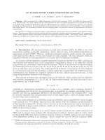
Fig. 5.1. Sets of the Taylor models before (Eq. (5.3)) and after shrink wrapping (Eq. (5.5)). The dotted line is the
boundary of the set that is described by the polynomial of the original Taylor model. The white area is the set described by
the original Taylor model, including the in terval term. The excess area introduced by shrink wrapping is shaded in grey.
Applying shrink wrapping in the linear model problem (5.1) is rather simple. For simplicity, let

us assume that shrink wrapping is performed in every integration step. Then we must compute [29]
q
j
:= 1 + d
j
/2, where
d
j
:= w

(T
j
)
−1
i
j


∞
.
12
If T is sufficiently well-conditioned, and if the interval terms are sufficiently small, then the factors d
j
are almost zero, and shrink wrapping is feasible for many integration steps.
The naive Taylor model method with shrink wrapping resembles the parallelepiped method. By
multiplying the non-constant coefficients of the Taylor polynomial, for linear autonomous ODEs the
interval term is absorbed as in the parallelepiped method. While T
j
is well-conditioned, d
j

is small,
and so is the excess area. On the other hand, q
j
(and the excess area) becomes large if T
j
becomes ill
conditioned, which is eventually the case if T has eigenvalues of different magnitude. In this case the
integration breaks down due to the growth of the Taylor polynomial coefficients.
The naive TM method with shrink wrapping is outlined as Algorithm 5.1.
Algorithm 5.1 (naive TM method with shrink wrapping)
Let the initial set be given as a Taylor model vector in m space variables.
For j := 0, 1 . . ., j
max
− 1:
1. Compute the m-dimensional Taylor model U = p
n
+ i (containing the flow of
the IVP at t
j+1
) as in the naive Taylor model method.
2. Absorb i into p
n
by shrink wrapping.
3. Continue the integration with the modified polynomial as the initial set for the
next time step.
5.3. Preconditioned Taylor Models. We showed in the previous section that shrink wrapping
has the s ame limitations as the parallelepiped method in traditional interval arithmetic. To make Taylor
model based integration successful for a larger class of IVPs, some stabilization proces s similar to the
QR interval method is required. For restoring good condition numbers of the maps defined by the linear
parts of the Taylor models in the integration process, Berz and Makino developed preconditioned Taylor

models [29].
In the naive Taylor model method with or without shrink wrapping, the flow of the ODE u

= f(t, u)
is represented by a single Taylor model at each grid point. In the preconditioned Taylor model method,
the flow of the ODE at t = t
j
is represented by a composition of a left and a right Taylor model
U
l
◦ U
r
= (p
l,j
+ i
l,j
) ◦ (p
r,j
+ i
r,j
).
Definition 5.2. The composition
U(x) :=

p
l
(x) + i
l

◦


p
r
(x) + i
r

(5.6)
of two Taylor models
U
l
(x) := p
l
(x) + i
l
, x ∈ x
l
,
U
r
(x) := p
r
(x) + i
r
, x ∈ x
r
,
is called a preconditioned Taylor model if
Rg (U
r
) ⊆ x

l
. (5.7)
The range enclosure condition (5.7) is essential in verified integration with preconditioned Taylor
models (s ee discussion below). The factorization into a left and a right Taylor model is not unique. Two
preconditioned Taylor models of the form (5.6) can have the same domain z and the same range, but
different polynomials and remainder intervals. In verified integration, preconditioning is used to replace
some representation of the flow at an intermediate grid point by a different set of initial values that is
more suitable for continuing the integration. Here preconditioning is essentially a substitution in space
variables. In the continuation of the integration, the right Taylor model is not involved at all. The
following theorem is a reformulation of a proposition given without a proof by Makino and Berz [29].
Taylor Model Based Integration of ODEs · August 18, 2006 13
Theorem 5.3. If the initial set of an IVP is given by a preconditioned Taylor model, then integrating
the flow of the ODE only acts on the left Taylor model.
For better understanding of this theorem, which is the key point of the preconditioned integration
method, we present first a formal proof, then an example with symbolic integration, and finally a
numerical example.
Proof. The space variables are parameters in the integration with respec t to time. If F(x, t) is a
primitive of f(x, t), that is if

f(x, t) dt = F(x, t),
then substituting x = g(u) does not affect F :

f(g(u), t) dt = F(g(u ), t).
Preconditioned integration uses x = (p
l,j
+ i
l,j
) and g(u) = (p
r,j
+ i

r,j
).
Example 5.4. Preconditioned symbolic integration over two time steps. We consider the IVP
x

= x(x + y), x(0) = 1 + a,
y

= −x(x + y), y(0) = −1 + b.
Its unique solution is
x(t) = (1 + a)e
(a+b)t
,
y(t) = a + b − (1 + a)e
(a+b)t
,
so that at t = 1,
x(1) = (1 + a)e
a+b
, y(1) = a + b − (1 + a)e
a+b
.
To continue the integration, we use the IVP
u

= u(u + v), u(0) = α,
v

= −u(u + v), v(0) = β
and obtain

u(1) = αe
α+β
, v(1) = α + β − αe
α+β
.
Due to the substitution rule, u(1) = x(2) and v(1) = y(2). Indeed, letting
α = (1 + a)e
a+b
,
β = a + b − (1 + a)e
a+b
,
we obtain
u(1) = (1 + a)e
2(a+b)
= x(2),
v(1) = (a + b) − (1 + a)e
2(a+b)
= y(2).
The same variable substitution as in Example 5.4 is applied when the initial set for an ODE is given
by some preconditioned Taylor model U
l
◦U
r
. To compute an enclosure of the flow, it suffices to integrate
the given ODE for the initial values defined by Rg (U
l
), and to compose the integrated Taylor model
with U
r

. If higher order terms appear in the composition process, they are included in the remainder
interval of the result, as in Example 2.2.
In practice, preconditioning is used to replace the integrated preconditioned flow at the end of the
j-th integration step,


U
l,j

◦ U
r,j
,
14
(where

U denotes integrated flow with respect to the given ODE) by a different preconditioned Taylor
model
U
l,j+1
◦ U
r,j+1
.
The initial set for the (j + 1)-st integration step is defined by Rg (U
l,j+1
). The method is s ucces sful if
• the amount of overestimation in the wrapping of


U
l,j


◦ U
r,j
by U
l,j+1
◦ U
r,j+1
is sufficiently
small, and if
• Rg (U
l,j+1
) is better suited for continuing the integration than

U
l,j
. For example, precondition-
ing can be used to reduce the condition number of certain matrices that control the propagation
of the global error (see example below), or to reduce the number of nonzero elements in the
polynomial part of the left Taylor model.
In Lohner’s QR-method, an ill-conditioned parallelepiped is wrapped by some well-conditioned m-
dimensional rectangle. For preconditioning Taylor models, a large variety of well-conditioned wraps
are conceivable. The optimal choice is still an open question for future research.
One important aspect of preconditioned integration is the computation of the remainder bounds in
the Picard iteration. If the initial set is given by (5.6), the validity of the enclosure is already guaranteed
if the remainder intervals hold for x ∈ Rg (U
r
). In practice, the remainder bounds are calculated for
x ∈ x, a larger set and a potential source of overestimation. In practical computations, overestimation
(loss of accuracy) is usually converted to costs (increase of computation time). A common strategy is to
limit the admissible size of the remainder intervals by some prescribed bound. Using a larger initial set

then has the effect of reducing step sizes and increasing overall computation time.
A simple choice for the left Taylor model (the initial set) in each integration step is a well-conditioned
linear map (a parallelepiped). The following description of preconditioned integration is a simplified
version of the presentation in [29]. We consider the linear autonomous IVP
u

= B u
u(0) = u
0
= c
0
+ C
0
x,
(5.8)
where B is a real matrix, c
0
is a real vector, C
0
is a diagonal matrix, and x is contained in [−1, 1]
m
. The
initial set is given by a Taylor model vector of the form (2.3). A suitable preconditioned Taylor model
for this initial set is
p
l,0
(x) = c
0
+ C
0

x, i
l,0
= 0, p
r,0
(x) = x, i
r,0
= 0.
We assume that the flow at t
j
is given by the preconditioned Taylor mo del
U
j
:= (p
l,j
+ i
l,j
) ◦ (p
r,j
+ i
r,j
) = (c
l,j
+ C
l,j
x + i
l,j
) ◦ (c
r,j
+ C
r,j

x + i
r,j
),
where c
l,j
and c
r,j
are real vectors, C
l,j
and C
r,j
are real matrices. Using the matrix T from Section 5.1,
the flow after integration is given by
U
j+1
:= (T c
l,j
+ T C
l,j
x + i
l,j+1
) ◦ (p
r,j
+ i
r,j
).
For c
l,j+1
:= T c
l,j

and any nonsingular matrix C
l,j+1
, the preconditioned Taylor model U
j+1
can be
rewritten as
U
j+1
= (T c
l,j
+ C
l,j+1
x + [0, 0]) ◦

C
−1
l,j+1
T C
l,j
x + C
−1
l,j+1
i
l,j+1

◦ (p
r,j
+ i
r,j
)


= (c
l,j+1
+ C
l,j+1
x + [0, 0]) ◦

C
−1
l,j+1
T C
l,j
x + C
−1
l,j+1
i
l,j+1

◦ (c
r,j
+ C
r,j
x + i
r,j
)

= (c
l,j+1
+ C
l,j+1

x + [0, 0]) ◦

C
−1
l,j+1
T C
l,j
(c
r,j
+ C
r,j
x + i
r,j
) + C
−1
l,j+1
i
l,j+1

= (c
l,j+1
+ C
l,j+1
x + [0, 0])
◦

C
−1
l,j+1
T C

l,j
c
r,j
+ C
−1
l,j+1
T C
l,j
C
r,j
x + C
−1
l,j+1
T C
l,j
i
r,j
+ C
−1
l,j+1
i
l,j+1

=: (c
l,j+1
+ C
l,j+1
x + [0, 0]) ◦ (c
r,j+1
+ C

r,j+1
x + i
r,j+1
).
Taylor Model Based Integration of ODEs · August 18, 2006 15
The interval term i
r,j
in the preconditioned Taylor model integration of (5.8) is propagated as the interval
term in the parallelepiped and QR interval iteration, if C
l,j+1
is chosen as in those methods. For C
l,j+1
=
T C
l,j
, the parallelepiped method is obtained, for T C
l,j
P
j
= Q
j
R
j
(where P
j
is a permutation matrix for
sorting the columns of T C
l,j
) and C
l,j+1

= Q
j
, the QR method. Numerical examples confirming these
relations are presented in Section 7.
For nonlinear ODEs, the nonlinear terms in the left Taylor model can be shifted to the right Taylor
model in the same manner [29]. However, the resulting Taylor model methods then differ from the
corresponding interval methods. First, the symbolic parts of the composed Taylor models describe
nonlinear enclosures sets of the flow, which need not be convex, in contrast to interval methods. Second,
the nonlinear terms in the left Taylor models then also act on the interval terms in the right Taylor
models. An analysis of the resulting interval propagation will be the subject of future research.
6. Preconditioned Quadratic Example. We now demonstrate QR preconditioned Taylor model
integration for the quadratic model problem of Section 4.1, namely
u

= v, u(0) ∈ [0.95, 1.05],
v

= u
2
, v(0) ∈ [−1.05, −0.95].
In each integration step, the left Taylor models are constructed via a QR factorization of the linear parts
of the integrated Taylor models of the previous integration step. As in the naive integration of this IVP
in Section 4.1, order n = 3 and step size h = 0.1 are used, and all numbers are displayed rounded to six
decimal digits.
In the first integration step, the initial set is described by the left Taylor model in space variables
at t
0
. The right Taylor model at t
0
is the identity map in space variables. Hence, the first integration

step is performed as in the naive Taylor model method (cf. Section 4.1), and we obtain the integrated
left Taylor models (4.3), namely

U
l,1
(a, b) := 0.904667 + 1.01a + 0.1b +

i
0
,

V
l,1
(a, b) := −0.909333 + 0.19a + 1.01b + 0.1a
2
+

j
0
,

a, b ∈ [−0.05, 0.05],
where

i
0
= [−5.09307E-5, 7.86167E-5],

j
0

= [−1.75707E-4, 1.60933E-4].
For reasons that will soon become clear, we normalize the domain such that a and b are contained in
[−1, 1]. Doing so (without changing the names of the variables), we have

U
l,1
(a, b) := 0.904667 + 0.0505a + 0.005b +

i
0
,

V
l,1
(a, b) := −0.909333 + 0.0095a + 0.0505b + 0.00025a
2
+

j
0
,

a, b ∈ [−1, 1].
So far, the right Taylor models have been unaffected by the integration process. Before continuing
the integration, however, we precondition the left Taylor models. We extract the linear parts of

U
l,1
and


V
l,1
, and obtain the matrix C
l,1
, from which we compute a QR factorization.
C
l,1
:=

0.0505 0.005
0.0095 0.0505

=

0.982762 −0.184876
0.184876 0.982762

·

0.0513858 0.0142500
0 0.0487051

=: QR.
The left Taylor models in the second integration step are built from the constant terms of

U
l,1
and

V

l,1
and from Q. Thus we get
U
l,1
(a, b) := 0.904667 + 0.982762a − 0.184876b,
V
l,1
(a, b) := −0.909333 + 0.184876a + 0.982762b.
The nonlinear term 0.00025a
2
in

V
l,1
and the interval terms

i
0
,

j
0
are collected in the right Taylor
models, which are multiplied by Q
T
. We obtain
Q
T
·


0
0.00025a
2

=

0.0000462190a
2
0.000245691a
2

16
and

i
0
j
0

:= Q
T
·


i
0

j
0


=

[−8.25368E-5, 1.07014E-4]
[−1.87213E-4, 1.67575E-4]

,
which yields
U
r,1
(a, b) := 0.0513858a + 0.0142500b + 0.0000462190a
2
+ i
0
,
V
r,1
(a, b) := 0.0487051b + 0.000245691a
2
+ j
0
,

a, b ∈ [−1, 1].
Before we can continue the integration, we must further modify the preconditioned Taylor models.
This is probably the most surprising part of the algorithm. It is also crucial for the validity of the
method. After the first time step, the flow of the IVP is contained in the composition of the left and
right Taylor models. For continuing the integration, we want to drop the right Taylor model. On one
hand, this is only feasible if the left Taylor model contains the flow of the IVP. On the other hand, the
set defined by the left Taylor model should not be much larger than the current flow, because that would
mean large overestimation. There are two potential solutions for ensuring the desired inclusion property.

We can either modify the domain of the independent variables, or we may modify the left Taylor model
by an additional transformation. We describe both alternatives in the following.
The starting point of the transformation is the range of the right Taylor model. We have
Rg

U
r,1

⊆ 0.0513858 · [−1, 1] + 0.0142500 · [−1, 1] + 0.0000462190 · [0, 1] + [−8.25368E-5, 1.07014E-4]
= [−0.0657183368, 0.065789033] ⊆ [−0.0657183, 0.0657890],
Rg

V
r,1

⊆ 0.0487051 · [−1, 1] + 0.000245691 · [0, 1] + [−1.87213E-4, 1.67575E-4]
= [−0.048892151, 0.049118366] ⊆ [−0.0488922, 0.0491184].
Thus we may continue the integration with the initial set for the second time step given by

U
l,1
(a, b) := 0.904667 + 0.982762a − 0.184876b,

V
l,1
(a, b) := −0.909333 + 0.184876a + 0.982762b,

a ∈ [−0.0657183, 0.0657890],
b ∈ [−0.0488922, 0.0491184]
(unchanged polynomials, but modified domain).

Alternatively, we can apply a linear transformation on the left and the right Taylor models by a
scaling matrix [29]. It is convenient here to denote the linear map (that is, a linear Taylor model S with
zero constant part and zero interval remainder term) associated with a matrix S by the matrix itself.
First note that for any nonsingular matrix S,
(U
l,1
, V
l,1
) ◦ (U
r,1
, V
r,1
) = (U
l,1
, V
l,1
) ◦ (S ◦ S
−1
) ◦ (U
r,1
, V
r,1
) ⊆ ((U
l,1
, V
l,1
) ◦ S) ◦ (S
−1
◦ (U
r,1

, V
r,1
)),
where the subset property is induced by the s ubdistributivity law of interval arithmetic [1, p. 3]. Letting
S :=

0.0657890 0
0 0.0491184

,
we obtain
(U
l,1
, V
l,1
) ◦ S =

0.904667
−0.909333

+

0.982762 −0.184876
0.184876 0.982762

0.0657890 0
0 0.0491184

a
b


=

0.904667
−0.909333

+

0.0646550 −0.00908081
0.0121628 0.0482716

a
b

.
Since S has been determined such that the range of each component of S
−1
◦ (U
r,1
, V
r,1
) is contained in
[−1, 1], it is feasible to continue the integration with the left Taylor models
U
l,1
(a, b) := 0.904667 + 0.0646550a − 0.00908081b,
V
l,1
(a, b) := −0.909333 + 0.0121628a + 0.0482716b,


a, b ∈ [−1, 1]
Taylor Model Based Integration of ODEs · August 18, 2006 17
as initial set for the second time step (modified polynomials, but original domain). The corresponding
right Taylor models are

U
r,1
V
r,1

:= S
−1
◦ (U
r,1
, V
r,1
) =

15.2001 0
0 20.3590

0.0513858a + 0.01425b + 0.000046219a
2
+
i
0
0.0487051b + 0.000245691a
2
+ j
0


=

0.781070a + 0.216602b + 0.000702534a
2
+ [−0.00125457, 0.00162662]
0.991586b + 0.00500202a
2
+ [−0.00381146, 0.00341165]

.
Remark 6.1. From a mathematical viewpoint, modification of the domain or of the polynomials
are equivalent approaches for factorizing preconditioned Taylor models, but maintaining the integration
domain via the scaling matrices is advantageous for the software implementation of the method, because
it simplifies the estimation of the higher order terms in the integration step.
In the second integration step, we use the initial set defined by U
l,1
and V
l,1
. Proceeding as before,
we obtain the integrated left Taylor models (for a, b ∈ [−1, 1])

U
l,2
(a, b) := 0.817551 + 0.0664561a − 0.00433580b +

i
1
,


V
l,2
(a, b) := −0.835195 + 0.0233831a + 0.0471479b
+0.000418026a
2
− 0.000117424ab + 0.00000824612b
2
+

j
1
,
where

i
1
= [−5.72276E-5, 9.15947E-5],

j
1
= [−1.80914E-4, 1.80850E-4].
Finally, the flow at t
2
is made up by the composition of the integrated left Taylor models and the previous
right Taylor models. We have
U
2
(a, b) :=

U

l,2
(U
r,1
(a, b), V
r,1
(a, b)) = 0.817551 + 0.0519069a + 0.0100952b + 0.000025a
2
+ [−3.48708E-4, 4.09534E-4],
V
2
(a, b) :=

V
l,2
(U
r,1
(a, b), V
r,1
(a, b)) = −0.835195 + 0.0182638a + 0.0518160b + 0.000507287a
2
−0.0000505ab − 0.0000025b
2
+ [−4.38606E-4, 4.28392E-4],
where a, b ∈ [−1, 1].
Algorithm 6.1 (QR preconditioned Taylor model method)
Let the initial set be given as a preconditioned Taylor model vector U
l,0
◦ U
r,0
in

m space variables, with U
r,0
the identity map and symbolic variables in [−1, 1].
For j := 0, 1 . . ., j
max
− 1:
1. Integrate U
l,j
(containing the flow of the IVP at t
j
) as in the naive Taylor
model method. Denote the integrated left Taylor model (containing the flow
of the IVP at t
j+1
) by

U
l,j+1
. The flow is also contained in

U
l,l+1
◦ U
r,j
.
2. Replace

U
l,j+1
◦ U

r,j
by U
l,j+1
◦ U
r,j+1
:
(i) Compute the QR factorization of the linear part of

U
l,j+1
.
(ii) Shift all but the constant part of

U
l,j+1
to U
r,j
. Make Q the linear
part of

U
l,j+1
. Apply Q
−1
on U
r,j
.
(iii) Bound the range of the new U
r,j
.

(iv) Apply a scaling matrix S
j+1
on U
r,j
such that each component of the
range of U
r,j+1
:= S
−1
j+1
◦ U
r,j
is contained in [−1, 1] and spans [−1, 1]
approximately.
(v) Set U
l,j+1
:=

U
l,j+1
◦ S
j+1
.
18
Compared with the naive Taylor model integration performed in Section 4.1, the polynomial
coefficients are identical except for roundoff errors. This does not invalidate the computations, since all
roundoff errors are rigorously bounded by the interval terms. Even though preconditioned integration is
the superior method with respect to accuracy in the long run, the interval terms after two integration
steps are larger here. The advantage of preconditioning becomes only apparent after several integration
steps (see Section 6.1). Algorithm 6.1 summarizes the preconditioned Taylor model method with

domain normalization.
6.1. Numerical Comparison with the QR Interval Method. Finally, we compare the perfor-
mance of Lohner’s software AWA [21] with the COSY Infinity integrator written by Makino. We use the
quadratic model IVP (4.1) for the comparison. For the computation, Taylor expansions of order 18 were
used in both programs. In both programs, the QR method (QR preconditioning) is used. The computed
enclosure sets are shown in Figure 6.1.
-2
-1.5
-1
-0.5
0
0.5
1
-2 -1.5 -1 -0.5 0 0.5 1 1.5
-1.5
-1
-0.5
0
0.5
1
1.5
-1 -0.8 -0.6 -0.4 -0.2 0 0.2 0.4 0.6 0.8 1 1.2
Fig. 6.1. Integration of quadratic model IVP with AWA and COSY Infinity for t ∈ [0, 2.8] (left), and with COSY
Infinity for t ∈ [0, 6] (right). Enclosures of the flow are shown for t
k
= 0.4k, k = 0, 1, . . . . The solid line in each picture
belongs to the approximate solution that was computed w ith a Runge-Kutta method (for the model ODE with point initial
values).
In the left picture, integration is performed in the time interval [0, 2.8]. In the beginning, the
enclosures from AWA (rectangular boxes) and COSY Infinity (nonlinear sets) are of similar quality.

Near the end of the integration domain, the enclosures from AWA start exploding. While AWA aborts
integration at t = 3.75, COSY Infinity is able to continue the integration much longer (right picture;
enclosures of AWA are not shown). We attribute this to the ability of Taylor model methods to use
non-convex enclosure sets of the flow.
This example s hows that Taylor model methods may perform much better than interval methods
on some problems, but this is not always the case. For some problems, interval methods can be as
effective. Moreover, if they succeed, interval methods are often faster than Taylor model methods,
because symbolic computations with multivariate polynomials are expensive.
7. Linear Numerical Examples. We compare interval methods and Taylor model methods for
the linear autonomous ODE
u

= B u,
where B is a real 3 × 3 matrix. Numerical results are displayed for three different choices of B. In all
examples, the initial values
u
0
=


[0.999, 1.001]
[0.999, 1.001]
[0.999, 1.001]


.
were use d. The computations were performed with AWA and with the COSY Infinity integrator. In all
examples, order 12 was chosen for the Taylor polynomial. Using lower orders (6 and 9 were tested) gave
Taylor Model Based Integration of ODEs · August 18, 2006 19
less accurate results, using higher orders (15 was tested) increased the computation times, but not the

accuracy of the results. For integration with COSY Infinity, the minimal step size was set to 0.25.
In the tables, the following notation is used.
• AWA iv/AWA pe/AWA QR denote the direct interval method, the parallelepiped method and
the QR method, respectively.
• TM na/TM sw/TM QR denote the naive Taylor model method without shrink wrapping, the
naive Taylor model method with shrink wrapping, and the Taylor model method with QR
preconditioning, respectively.
The observed performance of the methods is in agreement with the theoretical considerations in this
paper. Naive Taylor model integration without shrink wrapping performs as the direct interval method
(except for Example 1), naive Taylor model integration with shrink wrapping like the parallelepiped
method, and QR preconditioned Taylor model integration sim ilar to the QR method.
We call two matrices A and B floating-point similar, if A is obtained from B by a similarity transform
executed in floating-point arithmetic. Floating-point similar matrices are denoted by A ≈ B. Intervals
are sometimes displayed using a short notation with upper and lower indexes. For example, 1.4
7301
5593
E-001
denotes the interval [0.145593,0.147301].
Example 7.1. Pure Contraction.
B =


−0.4375 0.0625 −0.2651650429
0.0625 −0.4375 −0.2651650429
−0.2651650429 −0.2651650429 −0.375


≈



−
1
2
0 0
0 −
3
4
0
0 0 0


B has three distinct real eigenvalues, so that B describes a contraction without rotation. For such
problems, the parallelepiped method is not well suited, because the matrices A
j
, which have to be
inverted, become nearly singular. The interval metho d breaks down, and the corresponding naive Taylor
model method with shrink wrapping computes a practically useless enclosure of the solution.
Metho d t
end
Steps y
1
(t
end
)
AWA iv 100 216 1.4
7301
5593
E-001
AWA pe 52.6 131 aborted
AWA QR 100 216 1.4

7301
5593
E-001
TM na 100 391 [−2.378E+26, 2.378E+26]
TM sw 100 272 [−2.282E+112, 2.282E+112]
TM QR 100 122 1.4
7301
5593
E-001
Table 7.1. Numerical results for Example 7.1.
The direct interval method succeeds here. We also would have expected the naive Taylor model method
without shrink wrapping to succeed. While the reason for its failure is not clear, it provides further evidence for
our judgement that this method is not very effective. Both the QR interval method and the QR preconditioned
Taylor model method succeed here.
Metho d t Steps y
1
(t
end
)
AWA iv 76.5 393 aborted
AWA pe 100 449 1.49
522
222
E+000
AWA QR 100 449 1.49
522
222
E+000
TM na 100 396 [−1.517E+45, 1.517E+45]
TM sw 100 343 1.49

522
222
E+000
TM QR 100 343 1.49
522
222
E+000
Table 7.2. Numerical results for Example 7.2.
Example 7.2. Pure Rotation.
B =


0 −0.7071067810 −0.5
0.7071067810 0 0.5
0.5 −0.5 0


≈


0 −1 0
1 0 0
0 0 0


20
B has eigenvalues ±i and 0. The flow of this IVP is a rotating interval box. As expected, the direct
interval method and the naive Taylor model method fail, whereas the parallelepiped method and the
naive Taylor model method with shrink wrapping (and also the QR based methods) succeed.
Example 7.3. Contraction and Rotation.

B =


−0.125 −0.8321067810 −0.3232233048
0.5821067810 −0.125 0.6767766952
0.6767766952 −0.3232233048 −0.25


≈


0 −1 0
1 0 0
0 0 −
1
2


In our last example, B has eigenvalues ±i and −1/2, so contraction and rotation are combined.
Here, the direct interval method and the naive Taylor model method are bound to fail because of the
rotation, whereas the contraction causes the parallelepiped method and the Taylor model method with
shrink wrapping to fail.
Metho d t Steps y
1
(t
end
)
AWA iv 85.5 507 aborted
AWA pe 75.2 404 aborted
AWA QR 100 516 1.34

862
592
E+000
TM na 100 397 [−1.605E+55, 1.605E+55]
TM sw 100 357 [−3.566E+106, 3.566E+106]
TM QR 100 362 1.34
862
592
E+000
Table 7.3. Numerical results for Example 7.3.
Only the QR based methods can successfully deal with both contraction and rotation of the initial
set. For these methods, the overestimation of the final flow is hardly noticeable. This agrees with the
general observation that the QR decomposition is a very effective tool in fighting the wrapping effect,
both for the interval method and for the preconditioned Taylor model method.
Conclusion. We have compared traditional enclosure methods with Taylor model based integration.
For the verified solution of initial value problems for ODEs, we have shown how Taylor model methods
benefit from symbolic computations. Increased flexibility in admissible boundary curves of enclosures is
an intrinsic advantage over traditional interval methods, not only for the solution of ODEs. In future
research, we hope to contribute to the further development and increased use of Taylor model methods.
Acknowledgements. The authors thank Martin Berz and Kyoko Makino for several very helpful
clarifying discussions on Taylor models, and for making the COSY Infinity integrator available. Our
thanks also go to the referees for helpful comm ents.
REFERENCES
[1] G. Alefeld and J. Herzberger, Introduction to Interval Computations, Academic Press, New York, 1983.
[2] M. Berz, From Taylor series to Taylor models, in AIP Conference Proceedings 405, 1997, pp. 1–23.
[3] , Cosy Infinity Version 8 reference manual, NSCL Technical Report MSUCL-1088, Michigan State University,
1998.
[4]
, COSY INFINITY. August 2006.
[5] M. Berz and G. Hoffst

¨
atter, Computation and application of Taylor polynomials with interval remainder bounds,
Reliable Computing, 4 (1998), pp. 83–97.
[6] M. Berz and K. Makino, Verified integration of ODEs and flows using differential algebraic methods on high-order
Taylor models, Reliable Computing, 4 (1998), pp. 361–369.
[7] , New methods for high-dimensional verified quadrature, Reliable Computing, 5 (1999), pp. 13–22.
[8] , Performance of Taylor model methods for validated integration of ODEs, Lecture Notes in Computer Science,
3732 (2006), pp. 65–73.
[9] G. F. Corliss, Survey of interval algorithms for ordinary differential equations, Appl. Math. Comput., 31 (1989),
pp. 112–120.
[10] , Guaranteed error bounds for ordinary differential equations, in Theory and Numerics of Ordinary and Partial
Differential Equations, M. Ainsworth, J. Levesley, W. A. Light, and M. Marletta, eds., Clarendon Press, Oxford,
1995.
[11] J P. Eckmann, H. Koch, and P. Wittwer, A computer-assisted proof of universality in area-preserving maps,
Memoirs of the AMS, 47 (1984).
[12] P. Eijgenraam, The Solution of Initial Value Problems Using Interval Arithmetic, Mathematical Centre Tracts No.
144, Stichting Mathematisch Centrum, 1981.
Taylor Model Based Integration of ODEs · August 18, 2006 21
[13] J. Hoefkens, M. Berz, and K. Makino, Verified high-order integration of DAEs and higher-order ODEs, in Scientific
Computing, Validated Numerics and Interval Methods, W. Kr¨amer and J. Wolff von Gudenberg, eds., Kluwer,
Dordrecht, Netherlands, 2001, pp. 281–292.
[14] L. Jaulin, M. Kieffer, O. Didrit, and E. Walter, Applied Interval Analysis, Springer, London, 2001 .
[15] E. Kaucher, Self-validating computation of ordinary and partial differential equations, in C om pute rarith meti c:
Scientific Computation and Programming Languages, E. Kaucher, U. Kulisch, and Ch. Ullri ch, eds., Teubner,
Stuttgart, 1987, pp. 221–254.
[16] E. W. Kaucher and W. L. Miranker, Self-Validating Numerics for Function Space Problems, Academic Press,
New York, 1984.
[17] R. Klatte, U. Kulisch, Ch. Lawo, M. Rauch, and A. Wiethoff, C-XSC: A C++ Class Library for Extended
Scientific Computing, Springer, Berlin, 1993.
[18] R. Klatte, U. Kulisch, M. Neaga, D. Ratz, and Ch. Ullrich, Pascal-XSC – Language Reference with Examples,

Springer, Berlin, 1992.
[19] W. K
¨
uhn, Rigorously computed orbits of dynamical systems without the wrapping effect, Computing, 61 (1998),
pp. 47–67.
[20] U. Kulisch and W. L. Miranker, Computer Arithmetic in Theory and Practice, Academic Press, New York, 1981.
[21] R. Lohner, Einschließung der L¨osung gew¨ohnlicher Anfangs- und Randwertaufgaben und Anwendungen, PhD thesis,
Universit¨at Karlsruhe, 1988.
[22]
, Computation of guaranteed solutions of ordinary initial and boundary value problems, in Computat ional
Ordinary Differential Equations, J. R. Cash and I. Gladwell, eds., Clarendon Press, Oxford, 1992, pp. 425–435.
[23] , On the ubiquity of the wrapping effect in the computation of error bounds, in Perspectives of Enclosure
Methods, U. Kulisch, R. Lohner, and A. Facius, eds., Springer, Wien, 2001, pp. 201–217.
[24] K. Makino, Rigorous analysis of nonlinear motion in particle accelerators, PhD thesis, Michigan State University,
1998.
[25] K. Makino and M. Berz, Remainder differential algebras and their applications, in Computational Differentiation:
Techniques, Applications and Tools, M. Berz, C. Bischof, G. Corliss, and A. Griewank, eds., SIAM, Philadelphia,
1996, pp. 63–74.
[26]
, COSY INFINITY version 8, Nuclear Instruments & Methods in Physics Research A, 427 (1999), pp. 338–343.
[27] , Efficient control of the dependency problem based on Taylor model methods, Reliable Computing, 5 (1999),
pp. 3–12.
[28] , Taylor models and other validated functional inclusion methods, Int. J. Pure Appl. Math., 4 (2003), pp. 379–
456.
[29] , Suppression of the wrapping effect by Taylor model-based validated integrators, MSU Report MSUHEP 40910,
Michigan State University, 2004.
[30] K. Makino, M. Berz, and Y. Kim, Range bounding with Taylor models - some case studies, WSEAS Transactions
on Mathematics, 3 (2004), pp. 137–145.
[31] R. E. Moore, The automatic analysis and control of error in digital computation based on the use of interval numbers,
in Error in Digital Computation, Vol. I, L. B. Rall, ed., John Wiley and Sons, New York, 1965, pp. 61–130.

[32]
, Automatic local coordinate transformations to reduce the growth of error bounds in interval computation of
solutions of ordinary differential equations, in Error in Digital Com put atio n, Vol. II, L. B. Rall, ed., John Wiley
and Sons, New York, 1965, pp. 103–140.
[33] , Interval Analysis, Prentice Hall, Englewood Cliffs, N.J., 1966.
[34] P. S. V. Nataraj and K. Kotecha, Global optimization with higher order inclusion function forms. Part 1: A
combined Taylor-Bernstein form, Reliable Computing, 10 (2004), pp. 27–44.
[35] N. S. Nedialkov, Computing rigorous bounds on the solution of an IVP for an ODE, PhD thesis, University of
Toronto, 1999.
[36] N. S. Nedialkov and K. R. Jackson, A new perspective on the wrapping effect in interval methods for initial value
problems for ordinary differential equations, in Perspe ctives of Enclosure Methods, U. Kulisch, R. Lohner, and
A. Facius, eds., Springer, Wien, 2001, pp. 219–264.
[37] , Some recent advances in validated methods for IVPs for ODEs, Appl. Numer. Math., 42 (2003), pp. 269 –284 .
[38] N. S. Nedialkov, K. R. Jackson, and G. F. Corliss, Validated solutions of initial value problems for ordinary
differential equations, Appl. Math. Comput., 105 (1999), pp. 21–68.
[39] N. S. Nedialkov, K. R. Jackson, an d J. Pryce, An effective high-order interval method for validating existence
and uniqueness of the solution of an IVP for an ODE, Reliable Computing, 7 (2001), pp. 449–465.
[40] M. Neher, Geometric series bounds for the local errors of Taylor methods for linear n-th order ODEs, in Symbolic
Algebraic Methods and Verification Methods, G. Alefeld, J. Rohn, S. Rump, and T. Yamamoto, eds., Springer,
Wien, 2001, pp. 183–193.
[41] A. Neumaier, Interval Methods for Systems of Equations, Cambridge University Press, Cambridge, 1990.
[42]
, Taylor forms – use and limits, Reliable Computing, 9 (2003), pp. 43–79.
[43] H. Ratschek and J. Rokne, Computer Methods for the Range of Functions, Ellis Horwood Limited, Chichester,
1984.
[44] R. Rihm,
¨
Uber Einschließungsverfahren f¨ur gew¨ohnliche Anfangswertprobleme und ihre Anwendung auf Differential-
gleichungen mit unstetiger rechter S eite, PhD thesis, Universit¨at Karlsruhe, Germany, 1993.
[45]

, Interval methods for initial value problems in ODEs, in Topics in Validated Computations, J. Herzberger,
ed., Elsevier, Amsterdam, 1994, pp. 173–207.
[46] H. J. Stetter, Validated solution of initial value problems for ODE, Notes Rep. Math. Sci. Eng., 7 (1990), pp. 171–
193.
[47] N. F. Stewart, A heuristic to reduce the wrapping effect in the numerical solution of x

= f(t, x), BIT, 11 (1971),
pp. 328–337.