08 TAYLOR MODELS AND OTHER VALIDATED FUNCTIONAL INCLUDING METHOD MAKINO & m BERZ
Bạn đang xem bản rút gọn của tài liệu. Xem và tải ngay bản đầy đủ của tài liệu tại đây (797.1 KB, 78 trang )
International Journal of Pure and Applied Mathematics
Volume 4
No. 4
2003, 379-456
TAYLOR MODELS AND OTHER VALIDATED
FUNCTIONAL INCLUSION METHODS
Kyoko Makino1 , Martin Berz2
§
1
Department of Physics
University of Illinois at Urbana-Champaign
1110 W. Green Street, Urbana, IL 61801-3080, USA
2
Department of Physics and Astronomy
Michigan State University
East Lansing, MI 48824, USA
e-mail:
Abstract: A detailed comparison between Taylor model methods and
other tools for validated computations is provided. Basic elements of the
Taylor model (TM) methods are reviewed, beginning with the arithmetic
for elementary operations and intrinsic functions. We discuss some of
the fundamental properties, including high approximation order and the
ability to control the dependency problem, and pointers to many of the
more advanced TM tools are provided. Aspects of the current implementation, and in particular the issue of floating point error control, are
discussed.
For the purpose of providing range enclosures, we compare with
modern versions of centered forms and mean value forms, as well as the
direct computation of remainder bounds by high-order interval automatic differentiation and show the advantages of the TM methods.
We also compare with the so-called boundary arithmetic (BA) of
Lanford, Eckmann, Wittwer, Koch et al., which was developed to prove
existence of fixed points in several comparatively small systems, and
the ultra-arithmetic (UA) developed by Kaucher, Miranker et al. which
Received: January 7, 2003
§
Correspondence author
c
° 2003 Academic Publications
380
K. Makino, M. Berz
was developed for the treatment of single variable ODEs and boundary
value problems as well as implicit equations. Both of these are not
Taylor methods and do not provide high-order enclosures, and they do
not support intrinsics and advanced tools for range bounding and ODE
integration.
A summary of the comparison of the various methods including a
table as well as an extensive list of references to relevant papers are
given.
AMS Subject Classification: 65L20, 65L06
Key Words: Taylor model methods, high approximation order, dependency problem, centered forms, mean value forms, boundary arithmetic,
ultra-arithmetic
1. Introduction
The Taylor model (TM) methods were originally developed to solve a
practical problem from the field of nonlinear dynamics, namely providing
range bounds for normal form defect functions[17]. These functions are
typically comprised of (computer generated) code lists involving 104 to
105 terms and usually have a large number of local extrema; to make
matters worse, they exhibit a very significant cancellation problem. The
normal form defect functions themselves are obtained from the highorder dependence of solutions of ODEs on initial conditions. In various
meetings and a large number of private discussions, the authors posed
this combined range bounding and integration problem to the interval
community as an interesting project. However, it was uniformly believed
that because of dependency problem in the normal form defect functions,
the dimensionality, and the need to determine high-order dependencies
on initial conditions in the ODE integration, the problem is intractable
through any of the tools known in the community. And indeed, the
attempt to apply various state of the art packages was not successful.
As a remedy to this problem, we developed the Taylor model approach as an augmentation to earlier work on high-order multivariate
automatic differentiation and the differential algebraic methods to solve
ODEs. Specifically, final variables in a code list are expressed in terms of
a high-order multivariate floating point Taylor polynomial of initial variables, plus a remainder bound accounting for the approximation error.
TAYLOR MODELS AND OTHER VALIDATED...
381
Over suitably small domains, the polynomial representation is naturally
free of most of the dependency problem that the underlying function
may have had. At each node of the code list, the remainder bound is
calculated in parallel to the floating point coefficients; since this only requires information about the current Taylor coefficients, its calculation
itself is also free of much of the dependency problem of the original code
list; details will become clear in the definition of the arithmetic and in
the various examples that will be provided.
For the purpose of motivation, consider the problem of studying the
behavior of the polynomial function
f (x) = −371.9362500 − 791.2465656 · x + 4044.944143 · x2
+ 978.1375167 · x3 − 16547.89280 · x4 + 22140.72827 · x5
− 9326.549359 · x6 − 3518.536872 · x7 + 4782.532296 · x8
− 1281.479440 · x9 − 283.4435875 · x10 + 202.6270915 · x11
− 16.17913459 · x12 − 8.883039020 · x13 + 1.575580173 · x14
+ 0.1245990848 · x15 − 0.03589148622 · x16
− 0.0001951095576 · x17 + 0.0002274682229 · x18
(1.1)
in a validated way over a sufficiently small range including the point x =
2. Because of the large coefficients and the alternating signs, a treatment
with interval arithmetic, or more advanced tools like centered forms,
will suffer from significant overestimation because of the cancellation of
terms. However, if before evaluation of the function, the function is first
re-expanded in powers of (x − 2), it assumes the following form
f (x) = −.1181179453 − 4.339394861 · (x − 2) − 23.05727974 · (x − 2)2
+ 14.04340823 · (x − 2)3 + 316.6727626 · (x − 2)4
+ 583.1235424 · (x − 2)5 − 157.0468495 · (x − 2)6
− 1261.784612 · (x − 2)7 − 858.7604751 · (x − 2)8
+ 271.5211596 · (x − 2)9 + 454.2310790 · (x − 2)10
+ 107.4309653 · (x − 2)11 − 33.62710460 · (x − 2)12
− 18.29248130 · (x − 2)13 − 1.838912469 · (x − 2)14
+ 0.3548444855 · (x − 2)15 + 0.09668534124 · (x − 2)16
+ 0.007993746467 · (x − 2)17 + 0.0002274682229 · (x − 2)18 .
382
K. Makino, M. Berz
For the sake of compactness, the coefficients are shown only to 10 digits.
It is apparent that now, an evaluation with a reasonably small interval
including 2 will provide a much better result, since the contributions
of the various higher orders decrease in importance, and hence the dependency effect which often leads to the dreadful increase of width of
intervals during evaluation is reduced. We forgo numerical details about
dependency at this point, but refer to a later discussion of the matter
(see Figure 5), where the behavior of the function is studied and analyzed in detail.
If it is desirable to limit the total amount of information, it is possible to bound the terms beyond a certain order into an interval and
henceforth deal only with the lower order part and this interval. For
example, if P12 (x − 2) is the polynomial comprised of orders 0 through
12 of f and we are interested in studying over the domain [1.9, 2.1], then
over this domain we can assert f (x) ∈ P12 (x − 2) + [−2 · 10−12 , 2 · 10−12 ].
Even in this truncated form, we can study much of the behavior of the
function; for example, range bounding will only incur an additional overestimation of about 10−12 , and integration can be done to that accuracy
as well. So we observe that the simple trick of re-expanding around a
suitable point greatly simplified the functional behavior for the purpose
of using validated methods.
Apparently the idea applies to any polynomial function, also in more
than one variables. It also easily generalizes to rational functions, since
these can be written as ordered pairs (P, Q) of polynomials that can be
studied separately. The ordered pairs can be added and multiplied in
the obvious way.
The Taylor model methods introduced in [112], [113] and discussed
below capitalize on this observation by representing any functional dependency in terms of a (Taylor) polynomial of sufficiently high order,
plus a small interval bound capturing the parts of the function that deviate from the polynomial. As such it is merely a validated extension of
automatic differentiation methods[63], [20], namely those of high order
in many variables [11], [14], [61]; or in a more general context, the fact
known to scientists of all backgrounds that locally, smooth functions can
be “well” represented by their Taylor expansion. The only, but of course
crucially important, augmentation lies in the fact that we will rigorously
quantify the meaning of “well”.
The remainder of the paper is structured as follows. First we present
TAYLOR MODELS AND OTHER VALIDATED...
383
an arithmetic that allows the computation of Taylor models for any computer representable function expressed in terms of elementary binary
operations and intrinsic functions. Subsequently, and more importantly,
algorithms are reviewed that allow to perform a variety of common analytical operations. These include efficient range bounding for global
optimization, integration of functions, ODEs, DAEs, determining inverses, solutions of fixed point problems and of implicit equations, and
a variety of others. Subsequently, we will compare the behavior of Taylor models (TM) with those a variety of other tools and approaches for
some of the typical applications. We will study the interval method (I),
as well as the more advanced inclusion methods of the centered form
(CF) and the mean value form (MF). We also compare with various
interval polynomial methods, the foundations of which were already discussed by Moore [128]. Specifically, we study the method of interval
automatic differentiation (IAD) to compute a Taylor polynomial and a
remainder bound, as well as the advanced interval polynomial methods
known as boundary arithmetic (BA) of Lanford, Eckmann, Wittwer and
Koch, as well as ultra-arithmetic (UA) by Kaucher and Miranker et al.
We conclude with a summary of the comparison of the various methods.
2. Taylor Model Arithmetic
In the following we provide an overview about the various aspects of
the Taylor model approach. As we shall see in the development of the
next sections, the Taylor model method has the following fundamental
properties:
1. The ability to provide enclosures of any function given by a finite
computer code list by a Taylor polynomial and a remainder bound
with a sharpness that scales with order (n + 1) of the width of the
domain.
2. The ability to alleviate the dependency problem in the calculation.
3. The ability to scale favorable to higher dimensional problems.
We begin with a review of the definitions of the basic operations.
Definition 1. (Taylor Model) Let f : D ⊂ Rv → R be a function
that is (n + 1) times continuously partially differentiable on an open set
384
K. Makino, M. Berz
containing the domain D. Let x0 be a point in D and P the n-th order
Taylor polynomial of f around x0 . Let I be an interval such that
f (x) ∈ P (x − x0 ) + I for all x ∈ D.
(2.1)
Then we call the pair (P, I) an n-th order Taylor model of f around x0
on D.
Apparently P + I encloses f between two hypersurfaces on D. As a
first step, we develop methods to calculate Taylor models from those of
smaller pieces.
Definition 2.
(Addition and Multiplication of Taylor Models)
Let T1,2 = (P1,2 , I1,2 ) be n-th order Taylor models around x0 over the
domain D. We define
T1 + T2 = (P1 + P2 , I1 + I2 )
T1 · T2 = (P1·2 , I1·2 )
where P1·2 is the part of the polynomial P1 · P2 up to order n and
I1·2 = B(Pe ) + B(P1 ) · I2 + B(P2 ) · I1 + I1 · I2
where Pe is the part of the polynomial P1 · P2 of orders (n+1) to 2n, and
B(P ) denotes a bound of P on the domain D. We demand that B(P )
is at least as sharp as direct interval evaluation of P (x − x0 ) on D.
We note that in many cases, even tighter bounding of B(P ) is possible.
Definition 3.
(Intrinsic Functions of Taylor Models) Let T =
(P, I) be a Taylor model of order n over the v-dimensional domain
D = [a, b] around the point x0 . We define intrinsic functions for the
Taylor models[112] by performing various manipulations that will allow
the computation of Taylor models for the intrinsics from those of the arguments. In the following, let f (x) ∈ P (x−x0 )+I be any function in the
¯
¯
Taylor model, and let cf = f (x0 ), and f be defined by f (x) = f (x) − cf .
¯
¯
¯
Likewise we define P by P (x − x0 ) = P (x − x0 ) − cf , so that (P , I) is a
¯. For the various intrinsics, we proceed as follows.
Taylor model for f
TAYLOR MODELS AND OTHER VALIDATED...
385
Exponential. We first write
¢
¡
¢
¡
¯
¯
exp(f (x)) = exp cf + f (x) = exp(cf ) · exp f (x)
½
1 ¯
1 ¯
¯
= exp(cf ) · 1 + f (x) + (f (x))2 + · · · + (f (x))k
2!
k!
ắ
Ă
Â
1
+
(2.2)
(f (x))k+1 exp à f (x) ,
(k + 1)!
where 0 < θ < 1. Taking k ≥ n, the part
ắ
ẵ
(x) + 1 (f (x))2 + Ã Ã Ã + 1 (f (x))n
exp(cf ) · 1 + f
2!
n!
¯
is merely a polynomial of f , of which we can obtain the Taylor model
via Taylor model addition and multiplication. The remainder part of
exp(f (x)), the expression
ẵ
1
exp(cf ) Ã
(f (x))n+1
(n + 1)!
ắ
Ă
Â
1
(x))k+1 exp θ · f (x) , (2.3)
+··· +
(f
(k + 1)!
will be bounded by an interval. One first observes that since the Taylor
¯
polynomial of f does not have a constant part, the (n + 1)-st through
¯
¯
(k + 1)-st powers of the Taylor model (P , I) of f will have vanishing
polynomial part, and thus so does the entire remainder part (2.3). The
remainder bound interval for the Lagrange remainder term
exp(cf )
¡
¢
1
¯
¯
(f (x))k+1 exp θ · f (x)
(k + 1)!
¯
¯
can be estimated because, for any x ∈ D, P (x − x0 ) ∈ B(P ), and
0 < θ < 1, and so
¡
¢ ¡
¢k+1
¯
¯
¯
(f (x))k+1 exp θ · f (x) ∈ B(P ) + I
Ă
Â
ì exp [0, 1] Ã (B(P ) + I) .
(2.4)
The evaluation of the “exp” term is mere standard interval arithmetic.
In the actual implementation, one may choose k = n for simplicity, but it
is not a priori clear which value of k would yield the sharpest enclosures.
386
K. Makino, M. Berz
Logarithm. Under the condition ∀x ∈ D, B(P (x − x0 ) + I) ⊂
(0, ∞), we first write as follows
¯
¯
¯
f (x) 1 (f (x))2
1 (f (x))k
−
+ · · · + (−1)k+1
cf
2 c2
k ck
f
f
¯(x))k+1
1 (f
1
+ (−1)k+2
(2.5)
¡
¢k+1 .
k+1
¯
k + 1 cf
1 + θ · f (x)/cf
log(f (x)) = log cf +
Again, evaluating the first line is mere Taylor model addition and multiplication, and the second line yields an interval contribution only, since
¯
¯
the Taylor model (P , I) of f , when raised to the (n + 1)-st power, vanishes and produces no polynomial part.
Multiplicative inverse. Under the condition ∀x ∈ D, 0 ∈ B(P (x−
/
x0 ) + I), we write as follows:
)
(
¯
¯
¯
(f (x))k
1
f (x) (f (x))2
1
· 1−
+
− · · · + (−1)k
=
f (x)
cf
cf
c2
ck
f
f
k+1
¯
(f (x))
1
+ (−1)k+1
(2.6)
¡
¢k+2
k+2
¯
cf
1 + θ · f (x)/cf
and again observe that, when evaluated in Taylor model arithmetic, the
second line merely yields an interval contribution.
Square root. Under the condition ∀x ∈ D, B(P (x − x0 ) + I) ⊂
(0, ∞), we first re-write the square root in the following way
(
¯
¯
p
1 f (x)
1 (f (x))2
√
f (x) = cf · 1 +
− 2
2 cf
2!2
c2
f
)
¯
(2k − 3)!! (f (x))k
+ · · · + (−1)k−1
k!2k
ck
f
¯
1
(2k − 1)!! (f (x))k+1
√
+ (−1)k cf ·
¡
¢k+1/2
k+1
k+1
(k + 1)!2
¯
cf
1 + θ · f (x)/cf
and evaluate in Taylor model arithmetic, obtaining a pure interval contribution from the remainder term.
TAYLOR MODELS AND OTHER VALIDATED...
387
Multiplicative inverse of square root. Under the condition ∀x ∈
D, B(P (x − x0 ) + I) ⊂ (0, ∞), we rewrite the expression
(
¯
¯
1
1 f (x) 3!! (f (x))2
1
p
+ 2
= √ · 1−
cf
2 cf
2!2
c2
f (x)
f
)
k
¯
k (2k − 1)!! (f (x))
+ · · · + (−1)
k!2k
ck
f
¯(x))k+1
1
1
(2k + 1)!! (f
+ (−1)k+1 √ ·
¡
¢k+3/2
k+1
k+1
cf (k + 1)!2
¯
cf
1 + θ · f (x)/cf
and evaluate in Taylor model arithmetic, obtaining a pure interval contribution from the remainder term.
Sine. We use the addition theorem and power series expansion of
the sine function and obtain
1
¯
¯
sin(f (x)) = sin(cf ) + cos(cf ) · f (x) − sin(cf ) · (f (x))2
2!
1
1
¯
¯
(f (x))k+1 · J,
− cos(cf ) · (f (x))3 + · · · +
3!
(k + 1)!
where
½
−J0 if mod(k, 4) = 1, 2,
J0
else,
½
¯
cos(cf + θ · f (x)) if k is even,
J0 =
¯
sin(cf + θ · f (x)) else,
J=
and evaluate in Taylor model arithmetic; the last term generates merely
an interval contribution.
Cosine. Similarly, we have
1
¯
¯
cos(f (x)) = cos(cf ) − sin(cf ) · f (x) − cos(cf ) · (f (x))2
2!
1
1
¯
¯
+ sin(cf ) · (f (x))3 + · · · +
(f (x))k+1 · J,
3!
(k + 1)!
where
½
−J0 if mod(k, 4) = 0, 1,
else,
J0
½
¯
sin(cf + θ · f (x)) if k is even,
J0 =
¯
cos(cf + θ · f (x)) else.
J=
388
K. Makino, M. Berz
Hyperbolic sine. In a similar vein, we have
1
¯
¯
sinh(f (x)) = sinh(cf ) + cosh(cf ) · f (x) + sinh(cf ) · (f (x))2
2!
1
1
¯
¯
(f (x))k+1 · J,
+ cosh(cf ) · (f (x))3 + · · · +
3!
(k + 1)!
where
J=
½
¯
cosh(cf + θ · f (x)) if k is even,
¯
sinh(cf + θ · f (x)) else.
Hyperbolic cosine. We write
1
¯
¯
cosh(f (x)) = cosh(cf ) + sinh(cf ) · f (x) + cosh(cf ) · (f (x))2
2!
1
1
¯
¯
(f (x))k+1 · J,
+ sinh(cf ) · (f (x))3 + · · · +
3!
(k + 1)!
where
J=
½
¯
sinh(cf + θ · f (x)) if k is even,
¯
cosh(cf + θ · f (x)) else.
Arcsine. Under the condition ∀x ∈ D, B(P (x−x0 )+I) ⊂ (−1, 1),
using an addition formula for the arcsine, we re-write
q
´
³
p
arcsin(f (x)) = arcsin(cf )+arcsin f (x) · 1 − c2 − cf · 1 − (f (x))2 .
f
Utilizing that
q
p
g(x) ≡ f (x) · 1 − c2 − cf · 1 − (f (x))2
f
does not have a constant part, we have
1
32
32 · 52
(g(x))3 + (g(x))5 +
(g(x))7
3!
5!
7!
1
+ ··· +
(g(x))k+1 · arcsin(k+1) (θ · g(x)),
(k + 1)!
arcsin(g(x)) = g(x) +
where
√
arcsin0 (a) = 1/ 1 − a2 ,
arcsin00 (a) = a/(1 − a2 )3/2 ,
TAYLOR MODELS AND OTHER VALIDATED...
389
arcsin(3) (a) = (1 + 2a2 )/(1 − a2 )5/2 , ...
A recursive formula for the higher order derivatives of arcsin
arcsin(k+2) (a) =
1
{(2k + 1)a arcsin(k+1) (a) + k2 arcsin(k) (a)}
2
1−a
is useful [132]. Then, evaluating in Taylor model arithmetic yields the
desired result, where again the terms involving θ only produce interval
contributions.
Arccosine. Use arccos(f (x)) = π/2 − arcsin(f (x)).
Arctangent. Using an addition formula for the arctangent, we have
ả
à
f (x) cf
.
arctan(f (x)) = arctan(cf ) + arctan
1 + cf · f (x)
Utilizing that
g(x) ≡
¯
f (x) − cf
f (x)
=
1 + cf · f (x)
1 + cf · f (x)
does not have a constant part, we obtain
1
arctan(g(x)) = g(x) − (g(x))3 +
3
1
(g(x))k+1
+···+
k+1
1
1
(g(x))5 − (g(x))7
5
7
³
³
π ´´
· cosk+1 (arctan(θ · g(x)) · sin (k + 1) · arctan(θ · g(x)) +
2
and proceed as usual.
Antiderivation. We note that a Taylor model for the integral with
respect to variable i of a function f can be obtained from the Taylor
model (P, I) of the function by merely integrating the part Pn−1 of order
up to n − 1 of the polynomial, and bounding the n-th order into the new
remainder bound. Specically, we have
àZ xi
ả
1
i (P, I) =
Pn−1 (x)dxi , (B(P − Pn−1 ) + I) · (bi − ai ) . (2.7)
0
Thus, given a Taylor model for a function f, the Taylor model intrinsic functions produce a Taylor models for the composition of the
respective intrinsic with f. Furthermore, we have the following result.
390
K. Makino, M. Berz
Theorem 1. (Taylor Model Scaling Theorem) Let f, g ∈ C n+1 (D)
and (Pf,h , If,h ) and (Pg,h , Ig,h ) be n-th order Taylor models for f and
g around xh on xh + [−h, h]v ⊂ D. Let the remainder bounds If,h and
Ig,h satisfy If,h = O(hn+1 ) and Ig,h = O(hn+1 ). Then the Taylor models
(Pf +g , If +g,h ) and (Pf ·g , If ·g,h ) for the sum and products of f and g
obtained via addition and multiplication of Taylor models satisfy
If +g,h = O(hn+1 ), and If ·g,h = O(hn+1 ).
(2.8)
Furthermore, let s be any of the intrinsic functions defined above, then
the Taylor model (Ps(f ) , Is(f ),h ) for s(f ) obtained by the above definition
satisfies
Is(f ),h = O(hn+1 ).
(2.9)
We say the Taylor model arithmetic has the (n + 1)-st order scaling
property.
Proof. The proof for the binary operations follows directly from the
definition of the remainder bounds for the binaries. Similarly, the proof
for the intrinsics follows because all intrinsics are composed of binary
operations as well as an additional interval, the width of which scales at
least with the (n + 1)-st power of a bound B of a function that scales
at least linearly with h.
Ô
Remark 1. (High Order Scaling Property) The high order scaling
property of Taylor model arithmetic states that a given function f can
be approximated by another function P (a polynomial) with an error
that scales with high order as the domain decreases. This approximation
statement follows standard mathematical practice. However, in the interval community it is customary to study another related but different
meaning of scaling: namely the behavior of the overestimation of a given
method to determine the range of a function. In the conventional interval community, this scaling property is important because intervals,
including range intervals, play a leading role. In the world of Taylor
model algorithms, the use of intervals themselves is much reduced, since
as a general rule, expressions are kept in Taylor model form as much as
possible, for example to retain the ability to suppress dependency. Thus
in general, the high order scaling property as stated in the previous theorem is the relevant one. This, however, applies only in a limited sense
to the question of range bounding; more about this matter below and
in [120].
TAYLOR MODELS AND OTHER VALIDATED...
391
Having defined the intrinsics of Taylor model arithmetic as above,
we can summarize the main property of Taylor model arithmetic in the
following theorem:
Theorem 2.
( FTTMA, Fundamental Theorem of Taylor Model
Arithmetic) Let the function f : Rv → Rv be described by a multivariate Taylor model Pf + If over the domain D ⊂ Rv . Let the function
g : Rv →R be given by a code list comprised of finitely many elementary
operations and intrinsic functions, and let g be defined over the range
of the Taylor model Pf , +If . Let P + I be the Taylor model obtained by
executing the code list for g, beginning with the Taylor model Pf + If .
Then P + I is a Taylor model for g ◦ f.
Furthermore, if the Taylor model of f has the (n + 1)-st order scaling
property, so does the resulting Taylor model for g.
Proof. The proof follows by induction over the code list of g from
the elementary properties of the Taylor model arithmetic.
Ô
As an elementary example for the use of Taylor model arithmetic, we
show some results of a computation of the function sin2 (exp(x + 1)) +
cos2 (exp(x+1)), executed with an implementation of Taylor model arithmetic as discussed in the next section. Of course the function is identical
to 1, but the validated methods cannot capitalize on this information;
so this function can serve as a good example to assess the tightness of
various enclosure schemes. The left picture in Figure 1 shows the result
of the enclosure of the function by intervals, mean value form, centered
form, and the result of the Taylor model range bounding algorithm for
the domains [−2−j , 2−j ] for j = 1, ..., 7; more comparisons about these
methods and Taylor models follow below. Also shown in the right picture are empirically computed approximation orders as a function of j.
Indeed it can be seen that the width of the computed higher order remainder intervals scale with order (n + 1) for Taylor models of order n,
until near the floor of machine precision, at which point rounding effects
dominate.
As a side note we also observe that in the representation of a function
through its Taylor model, it is apparent that some functions that can be
represented exactly by intervals cannot be represented exactly by Taylor models; a situation that also occurs with other advanced inclusion
tools like centered forms. As an example of this effect, we consider the
function f (x) = 1/x. Figure 2 shows the behavior of the TM method
392
K. Makino, M. Berz
2
1
3
6
0
9
12
-2
14
12
13
3
1
6
3
1
11
1
9
1
9
6
10
1
3
9
-12
-14
1
2
9
6
6
3
4
9
6
6
6
6
3
3
3
3
1
1
1
4
5
6
1
3
1
2
6
12
3
6
1
7
53
6
INTERVAL
CENTERED
MEAN VALUE
1 1ST ORDER TM
3 3RD ORDER TM
6 6TH ORDER TM
9 9TH ORDER TM
12 12TH ORDER TM
9
6
-8
12
EAO
log 10 q
8
3
6
-10
9
INTERVAL
CENTERED
MEAN VALUE
1ST ORDER TM
3RD ORDER TM
6TH ORDER TM
9TH ORDER TM
12TH ORDER TM
9
3
12
-6
1
3
6
9
12
12
3
-4
12
1
9
12
12
9
12
9
4
5
6
7
j
1
0
1
2
3
j
Figure 1: Overestimation q (left) and empirical approximation orders
(right) for the function sin2 (f ) + cos2 (f ), with f = exp(x + 1), in the
domain [−2−j , 2−j ].
of various orders in comparison to the interval method and the centered
form and mean value form for the domains 2+[−2−j , 2−j ] for j = 1, ..., 7.
Intervals represent the result exactly, while Taylor models produce overestimation. However, for higher orders, the overestimation produced by
Taylor models is significantly less than that produced by centered forms,
although it of course never reaches the accuracy of the interval representation. For completeness we note that the bounding of the polynomial
part is here done with the LDB method [120]. The order of approximation is shown on the right of the figure. Many more examples showing
the behavior of Taylor model methods can be found below.
3. Implementation of Taylor Model Arithmetic
In the following, we describe in detail the current implementation of
Taylor model arithmetic in version 8.1 of the code COSY INFINITY.
Since in the Taylor model approach, the coefficients are floating point
(FP) numbers, care must be taken that the inaccuracies of conventional
FP arithmetic are properly accounted for. Algorithmically the methods
are rather straightforward; however for practical use of the methods,
the more important question is that of the soundness of the actual implementation. Besides the tests performed in the development of the
TAYLOR MODELS AND OTHER VALIDATED...
0
13
1
1
3
5
1
1
5
1
7
107
3
9
CENTERED
MEAN VALUE
1ST ORDER TM LDB
3RD ORDER TM LDB
5TH ORDER TM LDB
7TH ORDER TM LDB
9TH ORDER TM LDB
7
3
5
7
8
3
5
3
5
9
-8
1
3
5
7
9
9
11
3
9
-6
log 10q
12
1
3
7
-4
9
1
7
EAO
-2
393
7
5
5
5
5
3
3
3
3
1
1
1
1
1
2
3
4
5
6
6
5
53
-10
1
3
5
7
9
-12
-14
INTERVAL
CENTERED
MEAN VALUE
1ST ORDER TM LDB
3RD ORDER TM LDB
5TH ORDER TM LDB
7TH ORDER TM LDB
9TH ORDER TM LDB
9
7
9
3
5
7
9
7
9
4
5
7
9
3
1
2
1
-16
1
2
3
4
5
6
7
0
1
j
j
Figure 2: Relative overestimation q (left) and empirical approximation order (right) for the function 1/x with LDB range bounder in
2 + [−2−j , 2−j ].
program, various other tests have been performed. Corliss and Yu performed extensive tests of the COSY interval tools by porting of COSY
interval results to Maple in binary format and comparison with Maple
computations with nearly 1000 digits of accuracy. Several thousand
cases that are to be considered particularly difficult as well as around
106 random tests spanning all orders of magnitude of allowed domains
of the intrinsics were performed[36]. Independently, Revol performed
around 108 random tests of the interval arithmetic by comparison with
a guaranteed precision library for elementary operations and intrinsic
functions[156]. In addition, Revol proved the soundness of the algorithms in the floating point coefficient treatment of the Taylor model
implementation and checked the actual coding [157].
Definition 4. (Admissible FP Arithmetic) We assume computation is performed in a floating point environment supporting the four
elementary operations ⊕, ⊗, Ä, ®. We call the arithmetic admissible if
there are two positive constants denoted
εu : underflow threshold,
εm : relative accuracy of elementary operations,
such that
1. If the FP numbers a, b are such that a ∗ b exceeds εu in magnitude,
394
K. Makino, M. Berz
then the product a ∗ b differs from the floating point multiplication
result a ⊗ b by not more than |a ⊗ b| ⊗ εm .
2. The sum a + b of FP numbers a and b differs from the floating
point addition result a ⊕ b by not more than max(|a|, |b|) ⊗ εm .
Definition 5. (Admissible Interval Arithmetic) We assume that
besides an admissible FP environment, there is an interval arithmetic
environment of four elementary operations ⊕, ⊗, Ä, ®, as well as a set
S of intrinsic functions. We call the interval arithmetic admissible if for
any two intervals [a1 , b1 ] and [a2 , b2 ] of floating point numbers and any
° ∈ {⊕, ⊗, Ä, ®} and corresponding real operation ◦ ∈ {+, ×, −, /},
we have
a[a1 , b1 ] ° [a2 , b2 ] ⊃ {x ◦ y|x ∈ [a1 , b1 ], y ∈ [a2 , b2 ]},
(3.1)
and furthermore, for any interval intrinsic s ∈ S representing the real
function s, we have
s([a, b]) ⊃ {s(x)|x ∈ [a, b]}.
(3.2)
For the specific purposes of Taylor model arithmetic, some additional considerations are necessary. First we note that combinatorial
arguments show [17] that the number of nonzero coefficients in a polynomial of order n in v variables cannot exceed (n+v)!/(n! · v!). Furthermore, as also shown in [17], the number of multiplications necessary to
determine all coefficients up to order n of the product polynomial of two
such polynomials cannot exceed (n + 2v)!/ (n! · (2v)!) .
Definition 6. (Taylor Model Arithmetic Constants) Let n and v
be the order and dimension of the Taylor model computation. Then we
fix constants denoted
εc : cutoff threshold,
e: contribution bound
such that
1. ε2 > εu
c
2. 2 ≥ e > 1 + 2 · εm · (n + 2v)!/ (n! · (2v)!)
TAYLOR MODELS AND OTHER VALIDATED...
395
We remark that in a conventional double precision floating point environment, typical values for the constants of the admissible FP arithmetic may be εu = 10−307 and εm = 10−15 . The Taylor arithmetic cutoff
threshold εc can be chosen over a wide possible range, but since it is later
used to control the number of coefficients actively retained in the Taylor
model arithmetic, a value not too far below εm , such as εc = 10−20 , is
a good choice for many cases. Furthermore, for essentially all practically
conceivable cases of n and v, the choice e = 2 is satisfactory, and this is
the number used in our implementation.
Under the assumption of the above properties of the floating point
arithmetic, interval arithmetic, and the Taylor model arithmetic constants, we now describe the algorithms for Taylor model arithmetic,
which will lead to the definition of admissible FP Taylor model arithmetic.
Storage. In the COSY implementation, a Taylor model T of order
n and dimension v is represented by a collection of nonzero floating point
coefficients ai , as well as two coding integers ni,1 and ni,2 that contain
unique information allowing to identify the term to which the coefficient
ai belongs. The coefficients are stored in an ordered list, sorted in increasing order first by size of ni,1 , and second, for each value of ni,1 ,
by size of ni,2 . For the purposes of our discussion, the details about the
meaning of the coding integers ni,1 and ni,2 is immaterial; we merely
note in passing that the efficiency of our implementation depends critically on them, and details can be found in [11]. There is also other
information stored in the Taylor model, in particular the information
of the expansion point and the domain, as well as various intermediate
bounds that are useful for the necessary computation of range bounds;
however this information is not critical for the further discussion. For
simplicity of the subsequent arguments, all coefficients are always stored
normalized to the interval [−1, 1] with expansion point 0.
Only coefficients ai exceeding the cutoff threshold εc in magnitude,
i.e. satisfying |ai | > εc , are retained. In many practical cases, this entails significant savings in space and execution time; more on how the
non-retained terms are treated is described below. Since by requirement, ε2 > εu , the multiplication of two retained coefficients can never
c
lead to underflow. Besides the coefficients and coding integers, each
TM also contains an interval I composed of two floating point numbers
representing rigorous enclosures of the remainder bound.
Error collection. In the elementary operations of Taylor models,
396
K. Makino, M. Berz
the errors due to floating point arithmetic are accumulated in a floating point “tallying variable” t which in the end is used to increase the
remainder bound interval I by an interval of the form e ⊗ εm ⊗ [−t, t].
The factor e assures a safe upper bound of all floating point errors of
adding up the (positive) contributions to t. Accounting for the error
through a single floating point variable t with the factor e · εm “factored
out” notably increases computational efficiency. In addition, there is a
“sweeping variable” s that will be used to absorb terms that fall below
the cutoff threshold εc and are thus not explicitly retained.
Scalar multiplication. The multiplication of a Taylor model T
with coefficients ai , coding integers (ni,1 , ni,2 ) and remainder bound
interval I with a floating point real number c is performed in the following manner. The tallying variable t and the sweeping variable s are
initialized to zero. Going through the list of terms in the Taylor polynomial, each floating point coefficient ai is multiplied by the floating point
number c to yield the floating point result bk = ai ⊗ c. The tallying
variable t is incremented by |bk |, accounting for the roundoff error in the
calculation of bk . If |bk | ≥ εc , the term will be included in the resulting polynomial, and k will be incremented. If |bk | < εc , the sweeping
variable s is incremented by |bk |. After all terms have been treated, the
total remainder bound of the result of the scalar multiplication is set to
be [c, c] ⊗ I ⊕ e ⊗ εm ⊗ [−t, t] ⊕ e ⊗ [−s, s], which is performed in outward
rounded interval arithmetic.
Addition. Addition of two Taylor models T (1) and T (2) with coef(1)
(2)
(1)
(1)
(2)
(2)
ficients ai and aj , coding integers (ni,1 , ni,2 ) and (nj,1 , nj,2 ), and remainder bounds I1 , I2 , respectively, is performed similar to the merging
of two ordered lists. The pointers i, j of the two lists and pointer of the
(1)
(1)
merged list k are initialized to 1. Then iteratively, the terms (ni,1 , ni,2 )
(2)
(2)
(1)
(1)
(2)
(2)
and (nj,1 , nj,2 ) are compared. In case (ni,1 , ni,2 ) 6= (nj,1 , nj,2 ), the term
that should come first according to the ordering is merely copied, and
(1)
(1)
(2)
(2)
its pointer as well as k are incremented. In case (ni,1 , ni,2 ) = (nj,1 , nj,2 ),
we proceed as follows. We determine the floating point coefficient bk =
(1)
(2)
(1)
(2)
ai ⊕ aj . To account for the error, we increment t by max(|ai |, |aj |).
If |bk | ≥ εc , the term will be included in the resulting polynomial, and k
will be incremented. If |bk | < εc , the sweeping variable s is incremented
by |bk |. Finally i, j are incremented by one. After both the lists of T (1)
and T (2) are completely transversed, the remainder bound is determined
via interval arithmetic as I1 ⊕ I2 ⊕ e ⊗ εm ⊗ [−t, t] ⊕ e ⊗ [−s, s], which
TAYLOR MODELS AND OTHER VALIDATED...
397
is performed in outward rounded interval arithmetic.
Multiplication. The multiplication of two Taylor models T (1) and
(1)
(2)
(1)
T (2) of order n with coefficients ai and aj and coding integers (ni,1 ,
(1)
(2)
(2)
ni,2 ) and (nj,1 , nj,2 ), respectively, is performed as follows. The contributions I to the remainder bound due to orders greater than n are
computed using interval arithmetic as outlined in [112]. Next, the terms
(2)
of the polynomial T (2) are sorted into pieces Tm of exact order m respectively. Then, each term in T (1) with order k is multiplied with all
those terms of T (2) of order (n − k) or less.
(1)
(1)
For each one of the contributions, using the coding integers (ni,1 , ni,2 )
(2)
(2)
and (nj,1 , nj,2 ), we determine the location l of the product using the
method described in [11]. We determine the floating point product
(1)
(2)
p = ai ⊗ aj of the coefficients. To account for the error, we increment t by |p|. We add the term p to the coefficient bl . To account for
the error, we increment t by max(|p|, |bl |).
After all monomial multiplications have been executed, all resulting total coefficients bl of the product polynomial will be studied for
sweeping. If |bl | ≥ εc , the term will be included in the resulting polynomial, and l will be incremented. If |bl | < εc , the sweeping variable
s is incremented by |bl |, but l will not be incremented, i.e. the term
is not retained. In the end, the remainder bound I is incremented by
e⊗εm ⊗[−t, t]⊕e⊗[−s, s] which is executed in outward rounded interval
arithmetic.
Intrinsic Functions. All intrinsic functions can be expressed as
linear combinations of monomials of Taylor models, plus an interval
remainder bound Ii [112]. The coefficients are obtained via interval
arithmetic, including elementary interval operations and interval intrinsic functions. The necessary scalar multiplications, additions, and multiplications are executed based on the previous algorithms, and in the
end the interval remainder bound Ii is added to the thus far accumulated
remainder bound.
Remark 2. (Floating Point Versus Interval Coefficients) One may
wonder why we are choosing to represent Taylor models via floating
point coefficients and then having to separately address floating point
errors instead of merely storing the coefficients as intervals. The main
reason for this is performance. Apparently the storage required is only
approximately half of what would be required with intervals, and so for
398
K. Makino, M. Berz
the same amount of storage, the accuracy of the representation can be
increased;in the one dimensional case,this amounts to twice the order as
would be possible with interval coefficients! Also, the amount of floating
point arithmetic necessary to perform validated computations is reduced
by about a factor of two compared to an interval implementation.
The various algorithms just discussed form the basis of a computer
implementation of Taylor model arithmetic:
Definition 7. (Admissible FP Taylor Model Arithmetic) We call
a Taylor model arithmetic admissible if it is based on an admissible FP
and interval arithmetic and it adheres to the algorithms for storage,
scalar multiplication, addition, multiplication, and intrinsic functions
described above.
Remark 3. (FP Taylor Model Arithmetic in COSY INFINITY )
The code COSY INFINITY contains an admissible Taylor model arithmetic in arbitrary order and in arbitrarily many variables. The code
consists of around 50, 000 lines of FORTRAN’ 77 source that also crosscompiles to standard C. It can be used in the environment of the COSY
language, as well as in F77 and C. It is also available as classes in F90
and C++. The code is highly optimized for performance in that any
overhead for addressing of polynomial coefficients amounts to less than
30 percent of the floating point arithmetic necessary for the coefficient
arithmetic [11]. It also has full sparsity support in that coefficients below the cutoff threshold do not contribute to execution time and storage.
Remark 4. (Verification and Validation of the COSY FP Taylor
Model Arithmetic) The FP TM arithmetic implemented in COSY is
currently being verified and validated by two outside groups [36], [156]
with a suite of challenging test problems. Independently, the validity of
the algorithms forming the core of theCOSY Taylor model FP algorithm
have been verified by Revol [157].
4. Taylor Model Algorithms
The above algorithms for Taylor model arithmetic assure that also in
a computer environment subject to floating point errors, any computations using Taylor models lead to rigorous enclosures, and we obtain the
following result.
TAYLOR MODELS AND OTHER VALIDATED...
399
Theorem 3.
(Taylor Model Enclosure Theorem) Let the function
v
v
f : R → R be contained within Pf + If over the domain D ⊂ Rv .
Let the function g : Rv → R be given by a code list comprised of
finitely many elementary operations and intrinsic functions, and let g
be defined over the range of an enclosure of Pf , +If . Let P + I be the
result obtained by executing the code list for g in admissible FP Taylor
model arithmetic, beginning with the Taylor model Pf + If . Then P + I
is an enclosure for g ◦ f over D.
Proof. The proof follows by induction over the code list of g from
the elementary properties of the Taylor model arithmetic.
Ô
Apparently the presence of the oating point errors entails that P is
not precisely the Taylor polynomial. In a similar fashion, also the scaling
properties of the remainder bound in a rigorous sense is lost. However,
these properties of Taylor models are retained in an approximate fashion.
Remark 5. (Influence of Floating Point Arithmetic) In the presence of floating point errors, the polynomial P will be a floating point
approximation of the Taylor polynomial of g ◦ f if Pf was an approximate Taylor polynomial for f. Furthermore, any (n + 1)-st order scaling
property for the remainder interval will prevail approximately until near
the floor of machine precision.
As an immediate consequence, we obtain the following:
Algorithm 1. (Range Bounding with Taylor Models)
Input: a finite code list involving elementary operations and intrinsics describing the function f over the multivariate domain box D
Output: an enclosure of f in a Taylor model Pf + If , and an interval
bound B(f ) for the range of f over D
1. Set up a Taylor model TI enclosing the identity function. This is
comprised of the linear multivariate polynomial P (x) = x plus the
remainder bound [0, 0].
2. Evaluate the code list for f in Taylor model arithmetic. As a
result, obtain Pf + If .
3. Bound the range B(Pf ) of the polynomial Pf , obtain a range
bound B(f ) for f as B(f ) = B(Pf ) + If .
400
K. Makino, M. Berz
Apparently the sharpness of the range bounding depends on the
method to obtain the bound of the polynomial B(Pf ).It turns out that in
many practical cases, even mere evaluation with intervals yields suitable
results that are significantly sharper than what can be obtained with
centered and mean value forms. Furthermore, there are various ways to
obtain sharper enclosures for B(Pf ) that in many cases asymptotically
lead to a scaling of the overall error with order (n + 1) [120].
Another nearly immediate algorithm is the following.
Algorithm 2. (Quadrature with Taylor Models)
Input: a finite code list involving elementary operations and intrinsics
describing the function f over the multivariate domain box D
R
Output: an enclosure of D f the sharpness of which scales with order
(n + 1) with D
1. Set up a Taylor model TI enclosing the identity function. This is
comprised of the linear multivariate polynomial P (x) = x plus the
remainder bound [0, 0].
2. Evaluate the code list for f in Taylor model arithmetic. As a
result, obtain P + I.
3. Integrate the polynomial by manipulation of coefficients to obtain
a primitive P I for R and insert the endpoints of D into P I to
P,
obtain the integral D P.
R
R
R
4. Obtain an enclosure for D f as D f ⊂ D P + |D| · I
Various applications of the method are described in detail in [25].
It is possible with relative ease to determine integrals in eight variables
with Taylor models of order 10, yielding a global sharpness that scales
with order 10.
There are several other Taylor model algorithms that we briefly summarize here; for full details, see the respective literature that is cited in
each algorithm.
Algorithm 3. (Solving Implicit Equations with Taylor Models)
Input: an n-th order multivariate Taylor model
Output: a domain box over which this Taylor model in invertible,
as well as an n-th order Taylor model enclosure for the inverse.
Described in detail in [21], [70], [69]. An example of the performance
is given below in Figure 13.
TAYLOR MODELS AND OTHER VALIDATED...
401
Algorithm 4. (Solving ODEs with Taylor Models)
Described in detail in [112], [24], [121].
Algorithm 5.
(Solving implicit ODEs and DAEs with Taylor
Models)
Described in detail in [69] as well as [72], [74].
Algorithm 6. (Complex Arithmetic with Taylor Models)
To this end, merely represent the analytic function f by a pair of
Taylor models in two variables (x, y). Since each of the components of
an analytic function is itself infinitely often differentiable as a function
of the real variables x and y, the Taylor model method can be applied to
them individually [144]. This yields enclosures in sets with a sharpness
that scales with order (n + 1), and alleviates the dependency problem.
In the following sections, comparisons with centered forms (CF) and
mean value forms (MF) for range bounding are performed, and comparisons with interval automatic differentiation (IAD), boundary arithmetic
(BA) and ultra arithmetic (UA) are given.
5. Centered and Mean Value Forms
It has recently been suggested that it would be useful to have a detailed comparison between Taylor models and the centered form (CF)
and mean value form (MF) [127], [100], [155], [98], [2], [1], [131] for range
bounding. Since the latter two usually provide sharper enclosures than
intervals and earlier comparisons of Taylor models were mostly with intervals, it was suspected that for mere range bounding, the performance
of Taylor models would be rather similar to CF and MF, which are
known to have the quadratic approximation property. In this section we
attempt a comparison based on what we believe to be a limited collection of meaningful examples. We compare with Taylor model methods
of various orders, and subsequent bounding schemes based on either
naive interval evaluation of the Taylor polynomial, or based on the linear dominated bounder LDB [120]. To increase the demand on the LDB
method, in all examples shown no domain subdivisions as utilized in the
various Bernstein-based schemes [133], [134] are allowed. Apparently
allowing subdivision before applying LDB would increase the applicability of LDB to larger domains. We observe that overall, Taylor models
suppress dependency much better than centered forms and mean value
402
K. Makino, M. Berz
forms, resulting in frequently much sharper inclusions. Furthermore, in
many cases the LDB method leads to higher order enclosures of estimated ranges.
All computations are performed using COSY for the Taylor models,
while intervals, centered forms, and slopes were evaluated using the implementation in the INTLAB toolbox for Matlab [165]. Specifically, we
used INTLAB Version 3.1 under Matlab Version 6. We believe we have
used the code in the proper way, although documentation is somewhat
terse; as the author puts it, “To be frankly, there is not much other
documentation about INTLAB. In every routine, of course, the functionality is documented. Otherwise, we think INTLAB code is much
self-explaining.”. However, we are less sure about whether our use is
near optimal; some of the multivariate centered form computations for
the normal form problem discussed below took 45 minutes of CPU time,
while the Taylor model evaluation of the same function even of order
seven could be done in about 20 seconds on the same machine.
We assess the behavior of various algorithms to bound functions with
a measure q of relative overestimation [141],
q=
(estimated range)-(exact range)
.
(exact range)
(5.1)
We provide logarithmic plots of q as a function of domain width for centered forms (CF), mean value forms (MF), and Taylor models of various
orders. Usually, the domain we study has the form D = x0 +[−2−j , 2−j ].
We also study the behavior of the linear dominated bounder LDB [120],
an enhancement to the Taylor model bounding that often provides for
sharper inclusions.
We will also determine empirical approximation orders (EAO) by
computing the magnitude of the local slopes of q in a logarithmic plot
and adding 1, i.e. EAO = 1 + |d (log(q)) /d (log(|D|))|. With this definition, the interval evaluation will commonly have EAO of 1, while centered forms and mean value forms will have order 2. However, in case the
function under consideration has vanishing slope at the point of interest,
q will be reduced by 1 (or possibly more) since the exact range width in
the denominator then scales with the second (or a higher) power of the
domain width. We usually list the EAO only until the floor of machine
precision is reached. We frequently also list the average empirical approximation order (AEAO) for various methods, which is obtained by
TAYLOR MODELS AND OTHER VALIDATED...
403
averaging the EAO data for the given method over all choices of the
domain width.
For notational simplicity, in the following pictures, results obtained
using interval evaluation will be denoted by the symbol ¡, reminiscent
of an interval box, while those obtained by the mean value form and
centered form will be denoted by the symbols ∇ and 4, reminiscent of
a gradient and a difference quotient, respectively. Taylor models will be
identified by numbers corresponding to their orders.
We begin our discussion with the study of a simple three dimensional
example function with modest dependency but overall rather innocent
behavior studied in [112]. The function has the form
4 tan(3y)
q
− 120 − 2x − 7z(1 + 2y)
6x
3x + x 7(x8)
ả
à
(3y + 13)2
6y
+
sinh 0.5 +
8y + 7
3z
5x tanh(0.9z)
√
− 20y sin(3z),
− 20z(2z − 5) +
5y
f1 (x, y, z) =
(5.2)
and the function is defined for 0 < x < 8, y > 0, and z 6= 0. We study
the behavior on the domain interval boxes (2, 1, 1)+ [−2−j , 2−j ]3 and
show the results in Figure 3. As a function of j, we show log10 (q) for
interval evaluation, centered and mean value form as well as TM range
bounding by mere interval evaluation of the Taylor polynomial, and TM
range bounding through LDB of orders 3, 6, and 9. We also plot the
EAO for both of these cases, and compute the AEAO.
It can be seen that all Taylor model methods achieve enclosures
that are significantly sharper than CF and MF, showing the ability of
the Taylor model method to suppress whatever dependency there is in
the function. Without LDB, the approximation order of CF, MF and
all TM methods is 2. CF uniformly provides slightly sharper enclosures
as MF, as is frequently observed. The first order Taylor model method
behaves similar to CF, and is in fact slightly superior. The higher order
Taylor models, while still showing order 2 scaling, provide enclosures
that is about 1 order of magnitude sharper than those of CF.
With LDB, the approximation order of the Taylor model of order n
increases to (n + 1), until the floor of machine precision is reached. At
the most favorable point, the sharpness of the 9-th order Taylor model
method is about 11 orders of magnitude higher than that of CF.