24 monte carlo pengeny 2002
Bạn đang xem bản rút gọn của tài liệu. Xem và tải ngay bản đầy đủ của tài liệu tại đây (62.3 KB, 18 trang )
MONTE CARLO METHODS
Jonathan Pengelly
February 26, 2002
1 Introduction
This tutorial describes numerical methods that are known as Monte Carlo methods.
It starts with a basic description of the principles of Monte Carlo methods. It then
discusses four individual Monte Carlo methods, describing each individual method
and illustrating their use in calculating an integral. These four methods have been
implemented in my example program 8.2, and the results from these are used in
my discussion on each method. This discussion looks at the principles behind each
method. It also looks at the approximation error for each method and compares
each different method’s approximation accuracy. After this, the tutorial discusses
how Monte Carlo methods can be used for many different types of problem, that
are often not so obviously suitable to Monte Carlo methods. We then discuss the
reasons why Monte Carlo is used, attempting to illustrate the advantages of this
group of methods. Finally, I discuss how Monte Carlo methods relate to the field
of Computer Vision and give examples of Computer Vision applications that use
some form of Monte Carlo methods. Note that the appendix includes a basic math-
ematics overview, the program code and results that are refered to in section 3 and
some focus questions involving Monte Carlo methods. This tutorial does contain
a moderate content of mathematical and statistical concepts and syntax. The basic
mathematics overview is an attempt to describe some of the more familiar concepts
and syntax in relation to this tutorial and thus a quick initial review of this section
may improve the understandability and clarity of it.
2 Basic Description
Monte Carlo methods provide approximate solutions to a variety of mathematical
problems by performing statistical sampling experiments. They can be loosely de-
fined as statistical simulation methods, where statistical simulation is defined in
quite general terms to be any method that utilizes sequences of random numbers
1
to perform the simulation. Thus Monte Carlo methods are a collection of differ-
ent methods that all basically perform the same process. This process involves
performing many simulations using random numbers and probability to get an ap-
proximation of the answer to the problem. The defining characteristic of Monte
Carlo methods is its use of random numbers in its simulations. In fact, these meth-
ods derive their collective name from the fact that Monte Carlo, the capital of
Monaco, has many casinos and casino roulette wheels are a good example of a
random number generator.
The Monte Carlo simulation technique has formally existed since the early
1940s, where it had applications in research into nuclear fusion. However, only
with the increase in computer technology and power has the technique become
more widely used. This is because computers are now able to perform millions
of simulations much more efficiently and quickly than before. This is an impor-
tant factor because it means that the technique can provide an approximate answer
quickly and to a higher level of accuracy, because the more simulations that you
perform then the more accurate the approximation is (This point is illustrated in
the next section when we compare approximation error for different numbers of
simulations).
Note that these methods only provide a approximation of the answer. Thus
the analysis of the approximation error is a major factor to take into account when
evaluating answers from these methods. The attempt to minimise this error is the
reason there are so many different Monte Carlo methods. The various methods can
have different levels of accuracy for their answers, although often this can depend
on certain circumstances of the question and so some method’s level of accuracy
varies depending on the problem. This is illustrated well in the next section where
we investigate four different Monte Carlo methods and compare there answers and
the accuracy of their approximations.
3 Monte Carlo Techniques
One of the most important uses of Monte Carlo methods is in evaluating difficult
integrals. This is especially true of multi-dimensional integrals which have few
methods for computation and thus are suited to getting an approximation due to
their complexity. It is in these situations that Monte Carlo approximations become
a valuable tool to use, as it may be able to give a reasonable approximation in a
much quicker time in comparison to other formal techniques.
In this section, we look at four different Monte Carlo methods to approach
the problem of integral calculation. We investigate each method by giving a ba-
sic description of its individual procedure and then attempt to give a more formal
2
mathematical description. We also discuss the example program that is included
with this tutorial. It has implemented all four methods that we discuss, and also
has results from these different methods in integrating an example function.
Before we discuss our first method it must be brought to the reader’s atten-
tion the reasons why we are discussing four different Monte Carlo methods. The
first point in explaining this, is to acknowledge that there are many considerations
when using Monte Carlo techniques to perform approximations. One of the chief
concerns is to be able to get as accurate an approximation as possible. Thus, for
each method we discuss their associated error statistics (the variance is discussed).
There is also the consideration of what technique is most suitable to the problem
and so will get the best results. For example, a curve that has many plateaus (flat
sections) may be very suitable to a stratified sampling method because the flat sec-
tions will have very low variance. Thus, we discuss four different Monte Carlo
methods, because they all have their individual requirements and benefits. Prob-
ably the most important consideration, for the methods are the accuracy of their
approximations because the more accurate the approximation, the less samples are
needed to reach a specific level of accuracy.
3.1 Crude Monte Carlo
The first method for discussion is crude Monte Carlo. We are going to use this
technique to solve the integral I.
(1)
A basic description of this method is that you take a number, N, of random
samples where a ¡= s (sample value) ¡= b. For each random sample s, we find the
function value f(s) for the function f(x). We sum all of these values, and divide
by N to get the mean value from our samples. We then multiply this value by the
interval (b-a) to get the integral. This can be represented as -
(2)
Now, the next part to describe is the accuracy of this approximation technique,
because otherwise the answer will not be meaningful without a description of its
uncertainty. In my implementation, I did a very simple, one-dimensional example.
I found the variance of my sample by finding the mean of all of my N-groups
of samples. I then substituted the information into the equation to determine the
variance. The sample variance equation is -
3
(3)
Using this information you can determine the confidence intervals of your
method and determine how accurate your answer is. This information about our
implementation example, is discussed further on in the tutorial.
3.2 Acceptance - Rejection Monte Carlo
The next method for discussion is Acceptance - Rejection Monte Carlo. This is the
easiest technique to explain and understand. However, it is also the technique with
the least accurate approximation out of the four discussed.
A basic description of the Acceptance-Rejection method is that you have your
integral as before. In the (a,b) interval for any given value of x the function you
find the upper limit. You then enclose this interval with a rectangle that is high
enough to be above the upper limit, so we can be sure that the entire function for
this interval is within the rectangle. We now begin taking random points within the
rectangle and evaluate this point to see if it is below the curve or not. If the random
point is below the curve then it is treated as a successful sample. Thus, you take N
random points and perform this check, remembering to keep count of the number
of successful samples there have been. Now, once you have finished sampling,
you can approximate the integral for the interval (a,b) by finding the area of the
surrounding rectangle. You then multiply this area by the number of successful
samples over the total number of samples, and this will give you an approximation
of the integral for the interval (a,b). This is illustrated more clearly in the diagram.
Mathematically, we can say that the ratio of the area below the function f(x)
and the whole area of the rectangle (Max(f(x)) * (b-a)) is approximately the ratio of
the successful samples (k) and the whole number (N) of samples taken. Therefore
(4)
To find the accuracy of the approximation, I have used the same variance
technique as for the Crude Monte Carlo method. This analysis shows that the
Acceptance-Rejection method gives a less accurate approximation than crude monte
carlo.
3.3 Stratified Sampling
The basic principle of this technique is to divide the interval (a,b) up into subin-
tervals. You then perform a crude monte carlo approximation on each subinterval.
4
A
B
Figure 1: Acceptance-Rejection Monte Carlo method. We see the surrounding
rectangle (red lines) for the interval (a,b). We would now randomly sample points
within this rectangle to see if they are underneath the function line.
5
This is illustrated in this diagram.
The reason you might use this method is that now instead of finding the vari-
ance in one big go, you can find the variance by adding up the variances of each
subinterval. This may sound like you are just doing a long-winded performance
of the Crude Monte Carlo algorithm but if you have a function that is step-like or
that has periods of flat, then this method could be well-suited. This is because if
you did an integration of a sub-interval that was very flat then you are going to get
a very small variance value. Thus this is the advantage of the stratified sampling
method, you get to split the curve into parts that could have certain advantageous
properties when evaluating them on their own. Mathematically we can represent
the integration as -
(5)
Note that this equation is when the interval (a,b) has been broken into two
sub-intervals (a,c) and (c,b).
3.4 Importance Sampling
The last method we look at is importance sampling. This is the most difficult
technique to understand out of the four techniques. In fact, before any attempt to
explain the basic principles behind this method, we will discuss a sort of link from
the lasttechnique (stratified sampling) to theconcepts behind importance sampling.
Now in the figure we see that the four sub-intervals are quite different. I1
sees the value of f(x) staying very constant. However, as we progress across to
B, we see the value of f(x) becoming larger than the fairly steady curve of I1.
Now these larger values of f(x) are going to have more impact on the value of the
integral. So should we not do more samples in the area where there is the highest
values. By doing this, we will get a better approximation of a sub-interval that
contributes more to the integral than the other sub-intervals. We won’t skew the
results either, because you still have to get the total integral by adding every sub-
intervals together, all you have is a more accurateapproximation of an important
sub-interval of the curve.
This leads in to the method of importance sampling. This method gets its name
because it attempts to do more samples at the areas of the function that are more
important. The way it does this is by bringing in a probability distribution function
(pdf). All this is, is a function that attempts to say which areas of the function in
the interval should get more samples. It does this by having a higher probability in
that area. This diagram can be used as reference during my explanation.
6
A B
I1 I2 I3 I4
Figure 2: Stratified Sampling Monte Carlo method. This diagram sees the function
interval (a,b) divided into four equal sized intervals - (I1, I2, I3, I4).
7
A
B
f(x)
p(x)
Figure 3: Importance Sampling Monte Carlo method. Notice that this graph shows
both f(x) and a probability distribution function (p(x)).
8
Now first of all, note that we can define the integral equation as the following
because they are equal -
(6)
p(x) is the probability distribution function. Note that the integral of p(x) over
(a,b) is always equal to 1 and that for no value of x within the interval (a,b) will
p(x) evaluate to 0. The question is what do we do with p(x) now that we have put
it into the equation. Well, we can use it so that when perform our samples of the
curve f(x) within the interval (a,b), we can make the choices taking into account
the probability of that particular sample getting selected. For example, according
to the example graph about half of the probability curve area is in the last quarter
of the interval (a,b). Therefore, when we choose samples we should do it in a way
so that half of the samples get taken in this area of the interval.
Now, you may be wondering why we should do this? and how we can do it
without jeopardising the accuracy of our approximation? Well, the reason why we
should do this, is that if we have chosen a good probability distribution function,
then it should have a higher probability for samples to be selected at the important
parts of the interval (the parts where the values are highest). Thus, we will spend
more effort getting an accurate approximation of the important parts of the curve.
But, this will affect the accuracy of our approximation because we will hopefully
have a set of samples that focuses on certain parts of the curve. However, we coun-
teract this by giving the value of f(x) / p(x) for every individual sample. This acts
as a counterbalance to our unbalanced sampling technique. Thus the end result is
a Monte Carlo method that effectively samples the important parts of the curve (as
long as it is a good probability distribution function) and then scales this sampling
to give an approximation of the integral of f(x). Note again that the success of this
method in getting a more accurate approximation is entirely dependant on selecting
a good p(x). It has to be one that makes it more likely that a sample will be in an
area of the interval(a,b) where the curve f(x) has a higher than the average value
(and is thus more important to the approximation).
This method is effective in reducing error when it does have a good pdf because
it samples the important parts of the curve more (due to the increased probability of
a sample being selected in an important area). Thus it can get a good approximation
of these important parts which lowers variance because these important parts are
defined so because they have a larger effect on the overall approximation value.
9
3.5 Program Implementation and Discussion
These methods that are discussed previously are all important methods that do have
some key differences. The last two methods are able to improve the accuracy of
the approximations greatly, however they do need to have suitable conditions. In
the case of importance sampling, it needs a good probability distribution function
to come up with an effective approximation. In the case of stratified sampling it
can come up with a much more accurate approximation if the shape of the curve
is suitable and can be broken up into sections, with some being relatively flat thus
allowing a very accurate approximation for that sub-interval. The first two meth-
ods, which are really the two basic Monte Carlo methods, are important to know
as they both are used as the basis in more complex techniques.
The program implemented all four algorithms, and used them on the function
illustrated in the following figure.
Our results did agree with our predictions. The acceptance-rejection method
was the most inaccurate. Crude Monte Carlo was the next least effective approx-
imation model. Then the importance sampling model was next with the Stratified
Model being the most efficient model in my program. On reflection, this is a sen-
sible result, because the Stratified Model splits the interval into four sub-intervals
and two of these sub-intervals have a constant value of 1 (thus a variance of 0).
Another contributing factor is in the fact that my probability distribution function
models the function effectively enough but a better pdf would have resulted in more
accurate results.
Note that a full print out of the results and the program code is in the Appendix.
Here is a summary table of the variance results from the program. Note that in
my implementation, I also created a hybrid method which was based on the one
that I mentioned as a lead in to the discussion on Importance sampling. However,
the results for this method were disappointing, although I think it was a fault in
implementation because the method sounds feasible. I have included in the results
table, although I am sure it should be able to approximate better than the standard
stratified sampling model.
Implementation Results
Monte Carlo Method Variance
Crude Monte Carlo 0.022391
Acceptance/Rejection 0.046312
Stratified Sampling 0.011871
Hybrid Model 0.018739
Importance Sampling 0.0223
10
A
B
2
4
6
8
10
12
1
2 3
f(x)
p(x)
Figure 4: Program Implementation functions. f(x) is on the top. p(x) is on the
bottom.
11
4 Other Applications for Monte Carlo Techniques
The previous section went into detail about the use of various Monte Carlo meth-
ods to evaluate integrals. However Monte Carlo techniques can be applied to many
different forms of problems. In fact, Monte Carlo techniques are widely used in
physics and chemistry to simulate complex reactions and interactions. This section
is to illustrate the use of the basic Monte Carlo algorithm in another form of prob-
lem. It is a fairly simplistic example, however it illustrates Monte Carlo being used
from a different perspecitive. This form of problem can also be seen in the focus
questions in the appendix.
In this example, we have to imagine a coconut shy. We want to determine the
probability that if we take 10 shots at the coconut shy we will have an even number
of hits. The only fact that we know is that there is a 0.2 probability of having a hit
with a single shot. We can work out the answer to this question using Monte Carlo
by performing a large number of simulations of taking 10 shots at the coconut shy.
We can then count all of the simulations that have an even number of hits and put
that number over the total number of simulations. This gives us an approximation
of the probability of getting an even number of hits when we take 10 shys at the
coconuts.
This example illustrates the use of the Monte Carlo algorithm for a different
sort of problem. You may wonder where the use of random numbers is involved
in this process. Well, as we know the probability of getting a hit with a single
shot, we can use some random process to determine if each shot in each simulation
is successful. For example, we could use a random number between 0 and 1 to
simulate a shot at the coconuts. If the random number is between 0 and 0.2 then
we can call it a hit, otherwise we can count it as a loss. (Note that the probability
still stays at 0.2 to score a hit with a single shot). Thus now we can do all of the
simulations just by generating random numbers and using these as our single shots
at the coconuts.
Thus this is a simple illustration of using the principle behind Monte Carlo
methods and applying it to a different form of problem to come out with an effec-
tive approximation of the answer. Note that this example is so simple that Monte
Carlo techniques would not be a sensible choice in this situation because the actual
answer can be worked out with much less effort than performing a few hundred
thousand simulations. However Monte Carlo techniques are more valuable when
the problem is highly complex and where the effort required to get the actual an-
swer is larger than the amount of effort required to get a reasonable approximation
through simulation.
12
5 Why use Monte Carlo techniques?
Two of the main reasons why we use monte carlo methods are because of their anti-
aliasing properties and their ability to approximate quickly an answer that would
be very time-consuming to find out the answer too if we were using methods to
determine the exact answer.
This last point refers to the fact that Monte Carlo methods are used to simulate
problems that are too difficult and time-consuming to use other methods for. An
example is in the use of Monte Carlo techniques in intergrating very complex multi-
dimensional integrals. This is a task that other processes can not handle well, but
which Monte Carlo can.
The first point refers to the fact that since Monte Carlo methods involve a ran-
dom component in the algorithm, then this goes someway to avoiding the problems
of anti-aliasing (only for certain applications). An example that was brought to my
attention was that of finding the area of the black squares on a chess board. Now, if
I was using an acceptance-rejection method to attack this problem, I should come
out with a fair approximation, due to the fact that I would be going to random points
on the chessboard. However what would happen if I was trying to do the same pro-
cess but I used an algorithm that moved to a certain next point a set distance away
and then cotinued to do this, thus not having any random point selection. Well, the
potential problem is that this person may have a bad step size and may overevalu-
ate or underevaluate the number of successful trials he has, thus inevitably giving
a poor approximation.
These are two solid reasons why people use Monte Carlo techniques. Other
possible reasons could include its ease in simulating complex physical systems in
the fields of physics, engineering and chemistry.
6 How does this relate to Computer Vision?
Now from the above descriptions, we can see the value of Monte Carlo methods
are their ability to give reasonable approximations for problems that can be very
complex and time and resource consuming to solve. But how can this ability be
used in the field of Computer Vision?
The area of computer vision that I first found Monte Carlo methods being men-
tioned was object tracking. The article that I found used a Monte Carlo technique
discussed an algorithm called CONDENSATION - Conditional Density Propaga-
tion for Visual Tracking.
This technique was invented to handle the problem of tracking curves in dense
visual clutter. Thus it tracks outlines and features of foreground objects, modeled
13
as curves, as they move in substantial clutter, and in fact does this at a fairly quick,
efficient rate.
Basically, the algorithm has a cycle in which it is trying to predict the state
that the object is in. It models the state an object is in and then as the picture
moves ahead a frame, it trys to guess what likely states the object is now in. The
big advantage with this technique is that it keeps multiple hypothesis of the object
state open, thus allowing for a bit more flexibility with fixing incorrect guesses as
to the object state.
Now, the computer holds these guesses as to what the state is going to be as
probability distribution functions. In this case the areas of the curve with higher
probability are the states the computer thinks are going to be next. The last step is
where Monte Carlo Methods come into the procedure. This is where the computer
randomly samples from this probability distribution function (which is guessing at
the state of the object). It then checks these samples with image data to see if they
support any of the states of the object at all. The more accurate the sample, then
the more successfully weighted the sample response is.
Thus once you are finished taking the samples you now have the new proba-
bility distribution for the new frame of movement which will reflect the probable
parameter state that the object is in.
Another article that I found used Monte Carlo methods involved Object Recog-
nition. It used Monte Carlo methods to solve a complex integral that related back to
do with the probability that something was being falsely recognised as the object.
So, there are two examples of Computer Vision’s use for Monte Carlo methods.
I am sure that they have many applications in other areas of Computer Vision.
Especially, with their ability to give accurate approximations to complex integrals,
as integral calculus is used in many different areas of Computer Science.
7 Conclusion
Monte Carlo methods are a very broad area of mathematics. They allow us to get
reasonable approximations of very difficult problems through simulation and the
use of random numbers. I discussed four of these methods that can be used in
the evaluation of integrals. I then discussed my implementations of these methods
and discussed my program results. Finally, I gave two examples of Monte Carlo
methods being used within the field of Computer Science.
14
8 Appendix
8.1 Appendix A - Basic Mathematics Overview
8.1.1 Sigma Notation
(7)
The Greek letter, sigma, is very often used in mathematics to represent the sum
of a series. It is a shorthand notation. An example is -
(8)
This is shorthand for the series starting with the first term and ending with the tenth
term of 3n. Thus it equals = 3(1) + 3(2) + 3(3) + 3(4) + 3(5) + 3(6) + 3(7) + 3(8) +
3(9) + 3(10) = 165
The symbol 3n is called the summand, the numbers 1 and 9 are the limits of
the summation, and the symbol n is the index.
8.1.2 Variance and Standard Deviation
The variance is a measure of how spread out a distribution is. It is computed as the
average squared deviation of each number from its mean.
For example, for the numbers 1, 2, and 3 the mean is 2 and the variance is:
(9)
The formula for the variance in a population where m is the mean and N is the
number of scores is -
(10)
When the variance is computed in a sample you multiply by 1/(N-1) instead.
8.2 Appendix B - Program Code and Results
I have included my code and output from my program. It is attached to this tutorial.
15
8.3 Appendix C - Focus Question
8.3.1 Background
A student exits his COSC 453 lecture in a bewildered state. He is at position 4
on the map. He has four possible choices of direction in which to go but he is so
bewildered that he is equally likely to choose each direction (thus a probability of
0.25 of heading in any particular direction). Now at each position on the outside of
the map, the student will find an activity to do for the afternoon thus when a student
reaches one of these boundary positions he stops. The four points in the middle of
the map ( 4,5,8,9 ) the bewildered student is still looking for something to do for
the afternoon and once is equally likely to head in any one of the four directions
available (even back to the point he just came from).
8.3.2 Question
Using the Monte Carlo method, describe how you would find out an approximation
of the probability that a student leaving his COSC 453 lecture will find it to one of
the two pubs on the map.
8.3.3 Key
1 = Back to the flat
2 = Back to the graphics lab to do some study
3 = Back to the AI lab to do some study
4 = Starting position - A junction with four possible next moves
5 = A junction with four possible next moves
6 = Poppa’s Pizza to get some lunch
7 = Goes to the dental school for an appointment
8 = A junction with four possible next moves
9 = A junction with four possible next moves
10 = The Garden Sports Tavern (A pub)
11 = The Captain Cook (Also a pub)
12 = The Union to participate in a student protest
8.4 Appendix D - Project Sources
I have used a variety of sources to help develop my knowledge on Monte Carlo
methods. They could prove to be helpful for anybody looking to do some extra
reading on the topic. Here is a list of material that I have used but not directly
referenced.
16
11
12
1 2
3
4 5
6
7 8
9
10
Figure 5: Map of the states for the question. Note that each outside state is a
destination and is not able to be left.
17
Internet
- />- />- />Books
- Introduction to the Monte-Carlo Method, Author = Istvan Manno, Publisher
= AKADEMIAI KIADO, Budapest, Year = 1999
- The Monte Carlo Method, Editor = Yu. A. Shreider, Publisher = Pergamon
Press, Year = 1966
-The Monte Carlo Method of Evaluating Integrals, Author = Daniel T. Gille-
spie, Publisher = Naval Weapons Center, Year = 1975
18