Validating an a priori enclosure using high order taylor series
Bạn đang xem bản rút gọn của tài liệu. Xem và tải ngay bản đầy đủ của tài liệu tại đây (183.96 KB, 11 trang )
Validating an A Priori Enclosure Using
High-Order Taylor Series
George F. Corliss and Robert Rihm
Abstract
We use Taylor series plus an enclosure of the remainder term to validate the
existence of a unique solution for initial value problems in ordinary di erential
equations and to compute a coarse enclosure of that solution. The signi cance of
this result is its application to Lohner's AWA algorithm for validated solutions,
not to the theory of ordinary di erential equations. By using high-order Taylor
series in Lohner's Algorithm I, we are able to validate the solution over much
longer time steps than is done in the current AWA code. For Lohner's enclosure
by polynomials, the enclosures are expensive to compute, but it is easy to check
for enclosure. For our enclosure by Taylor series, the enclosures are free because
they are already being computed, but checking for enclosure requires 2 n polynomial root ndings. Work is continuing on an implementation that will allow
direct computational comparisons of the e ectiveness of the two methods.
Keywords: ordinary di erential equations, Lohner's algorithm, validated computation, Taylor series, enclosure methods.
0 Introduction
The AWA (Anfangswertaufgabe) program by Rudolf Lohner 4, 5, 6, 7, 8] computes
an enclosure of the solution of an initial value problem (IVP) in ordinary di erential
equations (ODE)
u0 = f (u); u(t0 ) = u0;
(1)
where we only know an interval enclosure u0] of the vector u0 in general. Without loss
of generality, Lohner assumes the system is autonomous only to simplify the proofs.
We assume that f is at least p ? 1 times continuously di erentiable in a domain D
with u0] D IR , p 2. Then there is a unique at least p times continuously
di erentiable solution u(t) in a neighborhood of t0.
AWA is a single-step method. At each integration time step, AWA applies two algorithms:
n
Algorithm I: (Existence and enclosure) Find a step size h and a coarse enclosure
interval u ] D such that for t 2 t ] := t ; t + h], the solution u(t) exists and
satis es u(t) 2 u ].
0
0
0
0
0
2
George F. Corliss and Robert Rihm
Algorithm II: (Tightening) Compute a tight enclosure for u(t) at t = t := t + h.
1
0
Throughout this paper, we use the term \validation" to mean \prove existence of u(t)
for some t and nd a coarse enclosure u0]".
The e ciency of AWA has been limited by the Euler step size enforced by Algorithm
I as used in the current program. We show that Taylor series plus an enclosure of the
remainder term can be used not only in Algorithm II to tighten the enclosure, but
also in Algorithm I for the validation step. The consequence of this result for AWA
is that Algorithm I can validate the existence of the unique solution over time steps
appropriate for high-order methods employed for tightening during Algorithm II.
The basic idea of AWA is to enclose the Taylor coe cients and the remainder term of
the solution. It goes back to Moore who presented his method in 1965 (see 10, 11]).
The Taylor coe cients are computed using recurrence relations derived from the ODE:
f (0) (u) := f (u);
(u)0
:= u;
( ?1)
( )
(2)
f (u) := @f@u f (u) ; i = 1; 2; : : :; p ? 1 ;
(u)
:= 1 f ( ?1) (u); i = 1; 2; : : :; p :
i
The recurrences given by Equation (2) are not as intimidating as they might appear;
this is just an expression of the computation of the Taylor coe cients for the solution.
They can be evaluated by using automatic di erentiation (see e.g. 12]).
If we begin the recurrences given by Equation (2) with the initial value u0 and compute
in exact arithmetic, we get the Taylor coe cients (u0 ) for the solution expanded at
t = t0 .
If we begin the recurrences given by Equation (2) with an interval vector u0] and
compute in rounded interval arithmetic, then we get enclosures ( u0]) of the Taylor
coe cients for all solutions starting from u0 2 u0].
We can also begin with a coarse interval u0] and compute the interval vectors ( u0]) .
Then (b ? t0 ) ( u0]) contains the remainder of the p ? 1st degree Taylor polynomial
t
of u(b), if u(t) 2 u0](t) for all t 2 t0 ; b].
t
t
We emphasize that the computation of these values does not pre-suppose the existence
of a solution. We are just computing sequences of numbers. If we cannot compute
any of these values, then we are not able to proceed with validation. However, if we
know an a priori enclosure u0] of the solution on t0], then
i
i
i
i
i
i
i
p
u(t) 2
u(t) 2
p
?1
X
p
i=0
p 1
(t ? t0) (u0 ) + (t ? t0 ) ( u0]) =: T (t; u0; u0]) or
?
X
i=0
i
p
i
p
p
(t ? t0) ( u0]) + (t ? t0 ) ( u ]) = T (t; u0]; u ]), resp.
i
i
p
0
p
p
0
(3)
Validating an A Priori Enclosure
3
for t 2 t0], if only the interval polynomial T stays in u0]. Moore as well as Lohner
use (modi cations of) this formula to tighten an a priori enclosure u0] (see e.g. 13]).
p
1 Current AWA Approach
Validation and the computation of a tight enclosure are separate, though related,
issues. This paper addresses only the issue of validation, the role of Lohner's Algorithm
I. The techniques of his Algorithm II for tightening the enclosure are discussed in
4, 5, 6, 7, 8]. Algorithm I uses the following theorem for validation.
Theorem 1 ( 6]) Let u ] D be an interval vector satisfying
0
?
u1] := u0 + 0; h] f u0]
Then
for t 2 t0 ] = t0; t0 + h].
u0 ] :
u(t) 2 u1] (and hence u(t) 2 u0])
It follows directly from
Theorem 2 Let u](t) and v](t) D be interval vector valued functions, and let each
p times continuously di erentiable function v(t) 2 v](t) satisfy
Zt
(v(t)) := u0 + f (v( )) d 2 u](t)
v](t)
(4)
t0
for t 2 t0 ]. Then the solution u of Equation (1) satis es
u(t) 2 u](t)
for t 2 t0 ].
Proof: If (4) holds and we start a Picard-Lindelof iteration
u (t) = (u ?1)(t)) = u0 +
(k )
Zt
(k
f (u( ?1) ( )) d ; k = 1; 2; : : :
k
t0
with a p times di erentiable function u(0) (t) 2 v](t), then every successor is again p
times di erentiable and lies in u](t). However, the sequence of Picard iterates should
leave this interval function if the solution did so.
4
George F. Corliss and Robert Rihm
It seems strange to let v(t) be p times di erentiable. However, this assumption is used
in the following section.
AWA nds a step size h and an interval u0] such that
?
? 0
u0] u1] := u0] + 0; h]f u0]
u] ;
(5)
for all t 2 t0 ] := t0; t0 + h], and hence validates that the solution of Equation (1) exists
on t0] and is contained in u0]. Figure 1 shows the a priori bound u0] = 0:2; 0:5] and
( u0 ]) for the logistic equation u0 = u(1 ? u), u(0) = 0:3, on the interval t 2 0; 0:6].
In this gure, ( u0]) u0] in the interval t 2 0; 0:5]. If we tighten u0] = 0:29; 0:5],
then ( u0]) u0] in the larger interval t 2 0; 0:563].
0.6
0.5
0.4
u 0.3
0.2
0.1
0
0
0.1
0.2
0.3
0.4
0.5
0.6
t
Figure 1. A priori bounds with u0] = 0:2; 0:5].
2 Lohner's Enclosure of u(p)
The allowable step size h for which validation can be done using Theorem 1 as described
in Section 1 is limited to a step appropriate for Euler's method, no matter how high
the order of the method used during Algorithm II to tighten the enclosure.
Stetter showed in 14] that for the problem u0 = Au, A 2 IR , the step size h
obtained by applying Theorem 1 may be multiplied by the degree p of the Taylor
n
n
Validating an A Priori Enclosure
5
polynomial used in Algorithm II. Algorithm II yields a validated tight enclosure for
t = t0 + ph because p!( u0]) = A u0] contains the p-th derivative u( ) (t) for all
t 2 t0; t0 + ph], even though u0] does not enclose the solution on this enlarged
interval, in general.
Lohner 9] suggests using coarse enclosures for higher derivatives also in the general
case. Actually, he uses Theorem 2 instead of Theorem 1 and a special kind of interval
polynomials for v](t) instead of a constant coarse enclosure as in the current AWA
program. Lohner guesses an enclosure v0 ] of u( ) (t)=p! satisfying
p
p
p
p
v](t) :=
?1
X
p
(t ? t0) (u0 ) + (t ? t0) v0 ] D:
i
p
i
i=0
The Picard-Lindelof operator reproduces the Taylor coe cients of the exact solution.
There is an interval vector v1 ] such that each p times di erentiable function v(t) 2
v](t) satis es
(v(t)) 2 u](t) :=
p?1
X
(t ? t0 ) (u0) + (t ? t0 ) v1 ]:
i
i
p
i=0
If v1] v0 ] holds, then we also have u](t) 2 v](t), and according to Theorem 2,
u(t) 2 u](t).
To obtain v1 ], one has to compute an enclosure of the remainder coe cient of the
p ? 2nd degree Taylor polynomial of f (v(t)) for all p times di erentiable functions
v(t) 2 v](t). It also contains the remainder coe cient of the p ? 1st degree Taylor
polynomial of (v(t)). For computing or enclosing these coe cients on a computer,
one has to apply polynomial interval machine arithmetic given by Eiermann 3], which
provides the enclosure of a xed number of Taylor coe cients of standard operations
and standard functions on interval polynomialsas well as the enclosure of the respective
remainders. The advantage of this idea of Lohner over the validation strategy discussed
in Section 1 is that validation is possible for step sizes appropriate for a method of
local order p.
Example 1 The solution of the initial value problem
u0 = ?u; u(0) = 1
satis es u(t) = e? 2 0; 1] for t 0. However, the application of Theorem 1 for
t
u ] = 0; 1] requires a step size 1 since
0
u0 + 0; h]f ( u0]) u0]
, 1 + 0; h](? 0; 1]) 0; 1]
, 0 h 1:
6
George F. Corliss and Robert Rihm
However, Lohner's approach yields validation for much longer steps. If we choose
p = 6 and v0 ] = 0; 1], we get
3
2
t4 t5 t6
v](t) = 1 ? t + t2 ? t6 + 24 ? 120 + 720 0; 1];
2
3
t4 t5
f ( v](t)) = ? v](t) ?1 + t ? t2 + t6 ? 24 + 120 1 ? h ; 1]; and
6
2
3
t4 t5 t6
u](t) = ( v](t)) = 1 ? t + t2 ? t6 + 24 ? 120 + 720 1 ? h ; 1]
6
for t 2 t0 ; t0 + h]. We have
1 ? h ; 1] v0 ] = 0; 1] , 0 h 6 :
6
Of course, we could enclose the sixth Taylor coe cient of f instead of the fth one to
obtain h = 7. However, in general we only assume f to be p ? 1 times di erentiable.
In this example, the coe cients of f (v(t)) can easily be calculated. However, there
is no implementation of the method for the general case yet, although Lohner has
described 9] such an implementation using the Eiermann operators for interval polynomial arithmetic.
3 Validated Enclosure Using Taylor Series
The use of Taylor series for validation, as well as for tight enclosure, is suggested by
pictures such as those in Figure 2, which shows Taylor series enclosures for the solution
of the Lorenz system.
20
18
16
14
12
10
8
6
4
2
0
0.01
0.02
0.03
t
0.04
0.05
Validating an A Priori Enclosure
7
30
20
10
0 0
0.01
0.02
0.03
0.04
0.05
0.03
0.04
0.05
t
-10
40
30
20
10
0
0
0.01
0.02
t
Figure 2. Taylor Series Enclosures for the Solution of the Lorenz System.
As already mentioned, AWA uses the recurrence relations (2) and the formula (3) for
computing a tight enclosure in Algorithm II after having validated a coarse enclosure
u0] for a step size h in Algorithm I. It would cause no additional costs if the Taylor
expansion (3) could also be used in Algorithm I. The following theorem shows that
this can actually be done.
Theorem 3 Let u 2 int( u ]) D. Let
0
0
u](t) :=
?1
X
p
(t ? t0) (u0 ) + (t ? t0 ) ( u0])
i
p
i
p
u 0] ;
(6)
i=0
for t 2 t0 ]. Then
u(t) 2 u](t) for t 2 t0] :
Proof: It follows from our assumptions that Equation (1) has a solution u in some
neighborhood of the point (t ; u ), for every u 2 u ]. We must prove that that
neighborhood includes all of t ]. If (6) holds, then u(t) 2 u](t) as long as u(t) 2 u ].
0
0
0
0
0
0
8
George F. Corliss and Robert Rihm
Assume that u(t) leaves u](t) =: u(t); u(t)], and hence u0] at b 2 int( t0]). Without
t
loss of generality, we assume u (b) = u (b) = sup u0] , for some j 2 f1; : : :; ng. From
t
t
u( ) (t) 2 p!( u0]) , it follows that
j
p
j
j
p
u0 (t) 2
?2
X
p
(t ? t0) (u0 ) + (t ? t0 ) ?1 p( u0]) ;
i
p
i
p
i=0
t
t
t
and hence u0 (t) u0 (t) on t0; b]. Therefore, u (b) = u (b) implies u (t) = u (t) for all
t 2 t0 ; b]. If u is constant, then we have u0 = u (b) = sup u0] , which contradicts
t
t
the assumption u0 2 int( u0]). Otherwise, u (b) is an isolated maximum of the p-th
t
degree polynomial u . The same holds for u (t), since this function is at least p times
continuously di erentiable in t0]. Hence, u(t) cannot leave u](t) at b.
t
j
j
j
j
j
j
j
j
j
j
This approach avoids complicated calculations and nevertheless takes the order p into
account. With p = 6, we can validate the coarse enclosure 0; 1] in Example 1 for
h = 2:1 , compared with h = 1 for a constant bound enclosure and h = 6 using
Lohner's polynomial enclosure.
Example 2 We want to validate the solution u(t) = 1=t of the initial value problem
u0 = ?u ; u(1) = 1
2
in the interval u0] = 0; 2]. For the constant bound enclosure, we have
u1] := 1 + 0; h](? 0; 2]2) = 1 ? 4h; 1]
u0] , h 1=4
as the maximal step size we can reach by applying Theorem 1. However, the approach
of this section for p = 2 yields a longer step:
u](t) = 1 ? (t ? 1) + 0; 8](t ? 1)2
p
1 + 33 0:42 :
16
0; 2] , h
4 Implications for AWA
Using the results of the previous section, AWA Algorithm I is
Task 1: Approximate solution. Compute Taylor coe cients of an approximate solution
u(t) :=
b
?1
X
p
(t ? t0) (u0 )
i
i
i=0
from recurrence relation (2). In practice, we must compute (u0) using rounded
interval arithmetic to capture any round-o errors. The work of Task 1 is already
being done in AWA Algorithm II.
i
Validating an A Priori Enclosure
9
Task 2: Guess a step h. Use heuristics based on the radius of convergence 1] of the
truncated series for u or on previous steps sizes.
b
Task 3: Guess a constant enclosure u0]. Bound the range of u( t0 ; t0 + h]), and in ate
b
it a little.
Task 4: Compute the remainder terms ( u0]) , for i = 0; : : :; p from the recurrence
relation (2). The work of Task 4 is already being done in AWA Algorithm II.
Task 5: Compute stepsize for validation. The stepsize is the point nearest to t0 (and
in t0]) at which
i
u](t) :=
p?1
X
(t ? t0 ) (u0) + (t ? t0) ( u0])
i
p
i
p
i=0
leaves u0]. This requires 2 n polynomial root ndings. For each polynomial root nding problem, it is su cient to compute only relatively coarse lower
bounds for the smallest real root in the interval (t0 ; t0 + h], so a few iterations
of a simpli ed interval Newton method should su ce.
Remark. Variable order. We must compute ( u ]) , : : :, ( u ]) ? in order to compute
0
0
0
p
1
( u ]) . Hence, it is relatively inexpensive to compute the step size in Task 5 for each
order p. The order used for validation in Algorithm I can be di erent from the order
used for tightening in Algorithm II. The information is readily available to make both
Algorithms I and II fully variable order.
Remark. Iteration. If Task 5 nds that u](t) u0] on t0], then we can repeat Tasks
4 and 5 with a larger h or else with u0] = u]( t0]).
Remark. Optimization. Given guesses for h from Task 2 and for u0] from Task
3, we compute in Task 5 the largest step for which we can validate existence and
containment. Numerical experiments have shown 2] that a carefully chosen u0] allows
step sizes 10 times as long as step sizes corresponding to u0] given by reasonable
heuristics. That suggests viewing Algorithm I as an optimization problem:
0
p
Maximize step size h
by varying guessed h and u0]
subject to u](t) :=
?1
X
p
(t ? t0 ) (u0) + (t ? t0) ( u0])
i
i
p
p
u0 ]
i=0
Remark. E ectiveness. Either Lohner's enclosure by polynomials or our enclosure by
Taylor series is signi cantly more expensive than Picard-Lindelof iteration of constant
bounds currently used by AWA. However, AWA Algorithm II involves the solution of
an ODE system of dimension n n, so almost any e ort we expend in Algorithm I
that allows AWA to take longer steps improves the overall e ciency of AWA.
10
George F. Corliss and Robert Rihm
Remark. Which is better? For Lohner's enclosure by polynomials, the enclosures
are expensive to compute, but it is easy to check for enclosure. For our enclosure by
Taylor series, the enclosures are free because they are already being computed, but
checking for enclosure requires 2 n polynomial root ndings. Work is continuing on an
implementation that will allow direct computational comparisons of the e ectiveness
of the two methods.
Acknowledgments
We thank the anonymous referee for helpful suggestions. The work of Corliss was
supported in part by National Science Foundation Grant No. DMS{9413525 and in
part by SUN Academic Equipment Grant No. EDUD{US{940208.
References
1] Y. F. Chang and G. Corliss, Solving Ordinary Di erential Equations Using
Taylor Series, ACM Trans. Math. Software, 8(1982), 114{144.
2] G. Corliss, Validating an A Priori Enclosure Using High-Order Taylor Series,
presented at SCAN '95, Wuppertal, 1995.
3] M. Ch. Eiermann, Adaptive Berechnung von Integraltransformationen mit
Fehlerschranken, PhD thesis, Universitat Freiburg, 1989.
4] R. J. Lohner, Anfangswertaufgaben im IR mit kompakten Mengen fur Anfangswerte und Parameter, Diplomarbeit, Inst. f. Angew. Math., Universitat Karlsruhe, 1978.
n
5] R. J. Lohner, Enclosing the Solutions of Ordinary Initial and Boundary Value
Problems, in Computer Arithmetic: Scienti c Computation and Programming
Languages, E. W. Kaucher, U. Kulisch, and C. Ullrich, eds., Wiley-Teubner Series
in Computer Science, Stuttgart, 1987, pp. 255{286.
6] R. J. Lohner, Einschlie ung der Losung gewohnlicher Anfangs{ und Randwertaufgaben und Anwendungen, PhD thesis, Universitat Karlsruhe, 1988.
7] R. J. Lohner, Interval Arithmetic in Staggered Correction Format, in Scienti c
Computing with Automatic Result Veri cation, E. Adams and U. Kulisch, eds.,
Academic Press, San Diego, 1993.
8] R. J. Lohner, On Step Size and Order Control in the Veri ed Solution of Ordinary
Initial Value Problems, presented at SCAN '93, September 1993, Vienna.
Validating an A Priori Enclosure
11
9] R. J. Lohner, Step Size and Order Control in the Veri ed Solution of IVP with
ODE's, presented at the SciCADE '95 International Conference on Scienti c Computation and Di erential Equations, Stanford, Calif., March 28 { April 1, 1995.
10] R. E. Moore, The Automatic Analysis and Control of Error in Digital Computation Based on the Use of Interval Numbers, in Error in Digital Computation,
Vol. I, L. B. Rall, ed., John Wiley and Sons, New York, 1965, pp. 61{130.
11] R. E. Moore, Interval Analysis, Prentice-Hall, Englewood Cli s, N.J., 1966.
12] L. B. Rall, Automatic Di erentiation: Techniques and Applications, vol. 120 of
Lecture Notes in Computer Science, Springer Verlag, Berlin, 1981.
13] R. Rihm, Interval Methods for Initial Value Problems in ODEs, in Topics in
Validated Computations, J. Herzberger, ed., Elsevier Science B.V., Amsterdam,
1994, pp. 173{207.
14] H. J. Stetter, Validated Solution of Initial Value Problems for ODE, in Computer Arithmetic and Self-Validating Numerical Methods Ch. Ullrich, ed., Academic Press, San Diego, 1990, pp. 171{186.
Addresses:
G.F. Corliss, Marquette University, Department of Mathematics, Statistics, and
Computer Science, P.O. Box 1881 Milwaukee, Wisconsin 53201-1881, USA.
R. Rihm, Universitat Karlsruhe, Institut fur Angewandte Mathematik, 76128 Karlsruhe, Germany.