vnode - A Validated Solver for Initial Value Problemsin Ordinary Differential Equations
Bạn đang xem bản rút gọn của tài liệu. Xem và tải ngay bản đầy đủ của tài liệu tại đây (1.05 MB, 218 trang )
VNODE-LP
A Validated Solver for Initial Value Problems
in Ordinary Differential Equations
Nedialko S. Nedialkov
Department of Computing and Software
McMaster University
Hamilton, Ontario, Canada
Technical Report CAS-06-06-NN
c
Nedialko S. Nedialkov, 2006
ii
Contents
Preface xi
I Introduction, Installation, Use 1
1 Introduction 3
1.1 The problem VNODE-LP solves . . . . . . . . . . . . . . . . . 3
1.2 On Literate Programming . . . . . . . . . . . . . . . . . . . . . 3
1.3 Applications . . . . . . . . . . . . . . . . . . . . . . . . . . . . . 4
1.4 Limitations . . . . . . . . . . . . . . . . . . . . . . . . . . . . . . 5
1.5 Prerequisites . . . . . . . . . . . . . . . . . . . . . . . . . . . . . 5
2 Installation 7
2.1 Prerequisites . . . . . . . . . . . . . . . . . . . . . . . . . . . . . 7
2.2 Successful installations . . . . . . . . . . . . . . . . . . . . . . . 7
2.3 Installation process . . . . . . . . . . . . . . . . . . . . . . . . . 8
2.3.1 Extracting the source code . . . . . . . . . . . . . . . . . . . . . 8
2.3.2 Preparing a configuration file . . . . . . . . . . . . . . . . . . . . 8
2.3.3 Building the VNODE-LP library and examples . . . . . . . . . 9
2.3.4 Installing the library files . . . . . . . . . . . . . . . . . . . . . . 10
3 Examples 13
3.1 Basic usage . . . . . . . . . . . . . . . . . . . . . . . . . . . . . . 13
3.1.1 Problem definition . . . . . . . . . . . . . . . . . . . . . . . . . . 13
3.1.2 Main pro gram . . . . . . . . . . . . . . . . . . . . . . . . . . . . 14
3.1.3 Files . . . . . . . . . . . . . . . . . . . . . . . . . . . . . . . . . . 16
3.1.4 Building an executable . . . . . . . . . . . . . . . . . . . . . . . 16
3.1.5 Output . . . . . . . . . . . . . . . . . . . . . . . . . . . . . . . . 17
3.1.6 Standard coding . . . . . . . . . . . . . . . . . . . . . . . . . . . 17
3.2 One-dimensional ODE . . . . . . . . . . . . . . . . . . . . . . . 19
3.3 Time-dependent ODE . . . . . . . . . . . . . . . . . . . . . . . . 20
3.4 Interval initial conditions . . . . . . . . . . . . . . . . . . . . . . 22
3.5 Producing intermediate results . . . . . . . . . . . . . . . . . . . 24
3.6 ODE control . . . . . . . . . . . . . . . . . . . . . . . . . . . . . 26
iii
iv Contents
3.6.1 Passing data to an ODE . . . . . . . . . . . . . . . . . . . . . . . 26
3.6.2 Integration with parameter change . . . . . . . . . . . . . . . . . 27
3.7 Integration control . . . . . . . . . . . . . . . . . . . . . . . . . 28
3.8 Wor k versus order . . . . . . . . . . . . . . . . . . . . . . . . . . 33
3.9 Wor k versus problem size . . . . . . . . . . . . . . . . . . . . . . 35
3.10 Stepsize behavior . . . . . . . . . . . . . . . . . . . . . . . . . . 36
3.11 Stiff problems . . . . . . . . . . . . . . . . . . . . . . . . . . . . 38
4 Interface 41
4.1 Interval data type . . . . . . . . . . . . . . . . . . . . . . . . . . 41
4.2 Wra pper functions . . . . . . . . . . . . . . . . . . . . . . . . . . 41
4.3 Interval vector . . . . . . . . . . . . . . . . . . . . . . . . . . . . 43
4.4 Solver’s public functions . . . . . . . . . . . . . . . . . . . . . . 43
4.4.1 Constructor . . . . . . . . . . . . . . . . . . . . . . . . . . . . . . 43
4.4.2 Integrator . . . . . . . . . . . . . . . . . . . . . . . . . . . . . . . 43
4.4.3 Set functions . . . . . . . . . . . . . . . . . . . . . . . . . . . . . 44
4.4.4 Get functions . . . . . . . . . . . . . . . . . . . . . . . . . . . . . 44
4.5 Constructing an AD object . . . . . . . . . . . . . . . . . . . . 45
4.6 Some helpful functions . . . . . . . . . . . . . . . . . . . . . . . 45
5 Testing 47
5.1 General tests . . . . . . . . . . . . . . . . . . . . . . . . . . . . . 47
5.2 Linear problems . . . . . . . . . . . . . . . . . . . . . . . . . . . 47
5.2.1 Constant coefficient problems . . . . . . . . . . . . . . . . . . . . 47
5.2.2 Time-dependent problems . . . . . . . . . . . . . . . . . . . . . . 48
5.3 Nonlinear problems . . . . . . . . . . . . . . . . . . . . . . . . . 49
6 Listings 51
II Third-party Components 59
7 Packages 6 1
8 IA package 63
8.1 Functions calling FILIB++ . . . . . . . . . . . . . . . . . . . . 63
8.2 Functions calling PROFIL . . . . . . . . . . . . . . . . . . . . . 65
9 Changing the rounding mode 69
9.1 Changing the rounding mode using FILIB++ . . . . . . . . . . 69
9.2 Changing the rounding mode using BIAS . . . . . . . . . . . . 70
III Linear Alg ebra and Related Functions 71
10 Vectors and Matrices 73
Contents v
11 Basic functions 75
11.1 Vector operations . . . . . . . . . . . . . . . . . . . . . . . . . . 75
11.2 Matrix/vector oper ations . . . . . . . . . . . . . . . . . . . . . . 78
11.3 Matrix operatio ns . . . . . . . . . . . . . . . . . . . . . . . . . . 78
11.4 Get/set column . . . . . . . . . . . . . . . . . . . . . . . . . . . 81
11.5 Conversions . . . . . . . . . . . . . . . . . . . . . . . . . . . . . 81
12 Interval functions 85
12.1 Inclusion . . . . . . . . . . . . . . . . . . . . . . . . . . . . . . . 85
12.2 Interior . . . . . . . . . . . . . . . . . . . . . . . . . . . . . . . . 85
12.3 Radius . . . . . . . . . . . . . . . . . . . . . . . . . . . . . . . . 86
12.4 Width . . . . . . . . . . . . . . . . . . . . . . . . . . . . . . . . 86
12.5 Midpoints . . . . . . . . . . . . . . . . . . . . . . . . . . . . . . 86
12.6 Intersection . . . . . . . . . . . . . . . . . . . . . . . . . . . . . 87
12.7 Computing h such that [0, h]a ⊆ b . . . . . . . . . . . . . . . . . 87
12.7.1 The interval case . . . . . . . . . . . . . . . . . . . . . . . . . . 87
12.7.2 The interval vector case . . . . . . . . . . . . . . . . . . . . . . 88
13 QR factorization 91
14 Matrix i nverse 93
14.1 Matrix inverse class . . . . . . . . . . . . . . . . . . . . . . . . . 93
14.2 Computing A
−1
. . . . . . . . . . . . . . . . . . . . . . . . . . . 94
14.3 Enclosing the solution of a linear system . . . . . . . . . . . . . 95
14.3.1 Initial box . . . . . . . . . . . . . . . . . . . . . . . . . . . . . . 96
14.3.2 Krawczyk’s itera tion . . . . . . . . . . . . . . . . . . . . . . . . 96
14.4 Enclosing the inverse of a general point matrix . . . . . . . . . . 97
14.5 Enclosing the inverse of an orthogonal matrix . . . . . . . . . . 99
14.6 Constructor and destructor . . . . . . . . . . . . . . . . . . . . . 99
IV Solver Implementation 101
15 Structure 103
16 Solution enclosure representation 105
16.1 Tight enclosure . . . . . . . . . . . . . . . . . . . . . . . . . . . 105
16.2 A priori enclosure . . . . . . . . . . . . . . . . . . . . . . . . . . 107
17 Taylor coefficient computation 109
17.1 Taylor coefficients for an ODE solution . . . . . . . . . . . . . . 109
17.2 Taylor coefficients for the solution of the variatio nal equation . . 110
17.3 AD class . . . . . . . . . . . . . . . . . . . . . . . . . . . . . . . 111
18 Control data 113
18.1 Indicator type . . . . . . . . . . . . . . . . . . . . . . . . . . . . 113
18.2 Interrupt type . . . . . . . . . . . . . . . . . . . . . . . . . . . . 113
vi Contents
18.3 Control data . . . . . . . . . . . . . . . . . . . . . . . . . . . . . 114
19 Computing a pri ori bounds 117
19.1 Theory background . . . . . . . . . . . . . . . . . . . . . . . . . 117
19.2 The HO E class . . . . . . . . . . . . . . . . . . . . . . . . . . . . 118
19.3 Implementation of the HOE method . . . . . . . . . . . . . . . . 119
19.3.1 Computing p
j
. . . . . . . . . . . . . . . . . . . . . . . . . . . . 119
19.3.2 Computing u
j
and
y
j
. . . . . . . . . . . . . . . . . . . . . . . 120
19.3.3 Computing a stepsize . . . . . . . . . . . . . . . . . . . . . . . . 121
19.3.4 For ming the time interval . . . . . . . . . . . . . . . . . . . . . 123
19.3.5 Selecting a trial stepsize for the next step . . . . . . . . . . . . 125
19.3.6 Computing a priori b ounds . . . . . . . . . . . . . . . . . . . . 125
19.4 Other functions . . . . . . . . . . . . . . . . . . . . . . . . . . . 12 6
19.4.1 Constructor and destructor . . . . . . . . . . . . . . . . . . . . 126
19.4.2 Accept a solution . . . . . . . . . . . . . . . . . . . . . . . . . . 127
19.4.3 Set functions . . . . . . . . . . . . . . . . . . . . . . . . . . . . 127
19.4.4 Get functions . . . . . . . . . . . . . . . . . . . . . . . . . . . . 128
19.4.5 Enclosing β . . . . . . . . . . . . . . . . . . . . . . . . . . . . . 128
20 Computing tight bounds on the solution 131
20.1 Theory background . . . . . . . . . . . . . . . . . . . . . . . . . 131
20.1.1 Predictor . . . . . . . . . . . . . . . . . . . . . . . . . . . . . . 131
20.1.2 Corrector . . . . . . . . . . . . . . . . . . . . . . . . . . . . . . 132
20.1.3 Computing a solution representation . . . . . . . . . . . . . . . 133
20.1.4 Computing Q
j+1
. . . . . . . . . . . . . . . . . . . . . . . . . . 134
20.2 Implementation . . . . . . . . . . . . . . . . . . . . . . . . . . . 134
20.2.1 The IHO class . . . . . . . . . . . . . . . . . . . . . . . . . . . . 134
20.2.2 Computing a tight enclos ure . . . . . . . . . . . . . . . . . . . . 135
20.2.3 Initialization . . . . . . . . . . . . . . . . . . . . . . . . . . . . . 135
20.2.4 Predictor . . . . . . . . . . . . . . . . . . . . . . . . . . . . . . 138
20.2.5 Corrector . . . . . . . . . . . . . . . . . . . . . . . . . . . . . . 140
20.2.6 Enclosure representation . . . . . . . . . . . . . . . . . . . . . . 147
20.2.7 Constructor . . . . . . . . . . . . . . . . . . . . . . . . . . . . . 151
20.2.8 Destructor . . . . . . . . . . . . . . . . . . . . . . . . . . . . . . 152
20.2.9 Accepting a solution . . . . . . . . . . . . . . . . . . . . . . . . 152
20.2.10 Set and get functions . . . . . . . . . . . . . . . . . . . . . . . 153
20.2.11 Constants . . . . . . . . . . . . . . . . . . . . . . . . . . . . . 153
20.2.12 Sorting columns of a matrix . . . . . . . . . . . . . . . . . . . 155
21 The VNODE class 159
21.1 Declaration . . . . . . . . . . . . . . . . . . . . . . . . . . . . . . 159
21.2 The integrator function . . . . . . . . . . . . . . . . . . . . . . . 160
21.2.1 Input c orrectness . . . . . . . . . . . . . . . . . . . . . . . . . . 160
21.2.2 Determine direction . . . . . . . . . . . . . . . . . . . . . . . . . 162
21.2.3 Initialization . . . . . . . . . . . . . . . . . . . . . . . . . . . . . 162
21.2.4 Methods involved in the initialization . . . . . . . . . . . . . . . 164
Contents vii
21.2.5 Validate existence and uniqueness . . . . . . . . . . . . . . . . . 166
21.2.6 Check last step . . . . . . . . . . . . . . . . . . . . . . . . . . . 166
21.2.7 Compute a tight enclosure . . . . . . . . . . . . . . . . . . . . . 169
21.2.8 Decide . . . . . . . . . . . . . . . . . . . . . . . . . . . . . . . . 169
21.3 Constructor/destructor . . . . . . . . . . . . . . . . . . . . . . . 170
21.4 Get functions . . . . . . . . . . . . . . . . . . . . . . . . . . . . 170
21.5 Set parameters . . . . . . . . . . . . . . . . . . . . . . . . . . . . 171
21.6 Files . . . . . . . . . . . . . . . . . . . . . . . . . . . . . . . . . 172
21.6.1 Interface . . . . . . . . . . . . . . . . . . . . . . . . . . . . . . . 172
21.6.2 Implementation . . . . . . . . . . . . . . . . . . . . . . . . . . . 173
21.7 Interfa c e to the VNODE-LP Package . . . . . . . . . . . . . . . 173
V AD Implementation 175
22 Using FADBAD++ 177
22.1 Computing ODE Taylor c oefficients . . . . . . . . . . . . . . . . 177
22.1.1 FadbadODE class . . . . . . . . . . . . . . . . . . . . . . . . . 177
22.1.2 Function description . . . . . . . . . . . . . . . . . . . . . . . . 178
22.1.3 Files . . . . . . . . . . . . . . . . . . . . . . . . . . . . . . . . . 179
22.2 Computing Taylor coefficients for the variational equation . . . 180
22.2.1 FadbadVarODE class . . . . . . . . . . . . . . . . . . . . . . 180
22.2.2 Function description . . . . . . . . . . . . . . . . . . . . . . . . 181
22.3 Files . . . . . . . . . . . . . . . . . . . . . . . . . . . . . . . . . 182
22.4 Encapsulated FADBAD++ AD . . . . . . . . . . . . . . . . . . 183
A Miscellaneous Functions 185
A.1 Vector output . . . . . . . . . . . . . . . . . . . . . . . . . . . . 185
A.2 Check if an interval is finite . . . . . . . . . . . . . . . . . . . . 185
A.3 Message printing . . . . . . . . . . . . . . . . . . . . . . . . . . . 186
A.4 Check intersection . . . . . . . . . . . . . . . . . . . . . . . . . . 186
A.5 Timing . . . . . . . . . . . . . . . . . . . . . . . . . . . . . . . . 188
Bibliography 189
viii Contents
List of Figures
1 Producing C++ and L
A
T
E
X files from cweb files . . . . . . . . . . . xi
2.1 Var iables of a VNODE-LP configuration file . . . . . . . . . . . . 9
2.2 File config/MacOSXWithProfil . . . . . . . . . . . . . . . . . . . 10
2.3 File config/LinuxWithProfil . . . . . . . . . . . . . . . . . . . . 11
2.4 The first six lines of makefile in vnodelp . . . . . . . . . . . . . . 12
3.1 makefile in vnodelp/user program . . . . . . . . . . . . . . . . . 16
3.2 The “standard” C++ code of basic.cc . . . . . . . . . . . . . . 18
3.3 Plots genera ted using integi.cc . . . . . . . . . . . . . . . . . . 24
3.4 Midpoints of the computed bounds with β = 8/3 from 0 to 20; and
with β = 8/3 changed to 5 at t = 10 . . . . . . . . . . . . . . . . . 29
3.5 Plots genera ted using integctrl.cc . . . . . . . . . . . . . . . . 32
3.6 Plots genera ted using orderstudy.cc . . . . . . . . . . . . . . . . 33
3.7 CPU time versus n for Problem 3.2. VNODE -LP takes 8 steps
for each n. . . . . . . . . . . . . . . . . . . . . . . . . . . . . . . . 36
3.8 Plots genera ted using orbit.cc . . . . . . . . . . . . . . . . . . . 37
3.9 Stepsize versus t on (3.8–3.9) for µ = 10, 10
2
, 10
3
, 10
4
. . . . . . . 39
6.1 The makefile in the examples directory . . . . . . . . . . . . . . 52
6.2 The gnuplot file for generating the plot in Figure 3.3 . . . . . . . 53
6.3 The matlab code for the DETEST E1 problem . . . . . . . . . . 54
6.4 The gnuplot file for generating the plots in Figure 3.4 . . . . . . . 54
6.5 The gnuplot file for generating the plots in Figure 3.5 . . . . . . . 55
6.6 The gnuplot file for generating the plots in Figure 3.6 . . . . . . . 56
6.7 The gnuplot file for generating the plots in Figure 3.7 . . . . . . . 57
6.8 The gnuplot file for generating the plots in Figure 3.8 . . . . . . . 57
6.9 The gnuplot file for generating the plots in Figure 3.9 . . . . . . . 58
15.1 Classes in VNODE -LP. The triangle arrows denote inheritance
relations; the nor mal arrows denote uses relations. . . . . . . . . . 104
21.1 The case t
end
⊆ T
j
. We set t
j+1
= t
tend
. . . . . . . . . . . . . . . 168
21.2 When close to t
end
, we ta ke the “middle” as the next integr ation
point. . . . . . . . . . . . . . . . . . . . . . . . . . . . . . . . . . . 169
ix
x List of Figures
Preface
We present VNODE-LP, a C++ solver for computing bounds on the solu-
tion of an initial-value problem (IVP) for an ordinary differential eq uation (ODE).
In contrast to traditional ODE solvers, which compute approximate solutions, this
solver proves that a unique solution to a problem exists and then computes rigor-
ous bounds that are guaranteed to contain it. Such bounds can be used to help
prove a theoretica l result, check if a solution satisfies a condition in a safety-critical
calculation, o r simply to verify the results produced by a traditional ODE solver.
This package is a successor of the VNODE [25], Validated Numerical ODE,
package of N. Nedialkov. A distinctive featur e of the present solver is that it is de-
veloped entirely using Literate Programming (LP) [17]. As a result, the correctness
of VNOD E-LP’s implementation can be examined much easier than the correct-
ness of VNODE—the theory, documentation, and sourc e code of VNODE-LP are
interwoven in this manuscript, which can b e verified for correctness by a human
exp ert, like in a peer-review process.
Literate programming. With LP, a program (or function) is normally subdivided
into pieces of code or chunks, and each of them may be subdivided into smaller
chunks. How they are divided and put together should be clear from the exposition.
The present document is produced by cweave [18] on L
A
T
E
X-like cweb files,
which contain both L
A
T
E
X text and C++ code. The C++ code fo r VNODE-LP
and all the exa mples are g enerated by running ctangle [18] on those files; see
Figure 1.
Figure 1. Producing C++ and L
A
T
E
X files from cweb files
Structure. Part I describes the problem VNODE-LP solves, shows how it can
xi
xii Preface
be installed, and illustrates on s e veral examples how VNODE-LP ca n be used.
Parts II–V contain the implementation of this package.
If a reader is interested only in using VNODE-LP, then studying Part I
should provide sufficient knowledge for using this package.
This document is open: errors found by a reader will be fixed and suggestions
on improving it will be incorporated. Such sugges tions can be on both exp osition
and code.
Acknowledgments. This work was supported in part by the Natural Sciences and
Engineering Research Council of Canada.
George Corliss has made many valuable comments on this manuscript. Dis-
cusssions with George Corlis, Baker Kearfott, John Pryce, and Spencer Smith have
resulted in va rious improvements of the presentation.
N. Nedialkov
July 26, 2 006
Part I
Introduction, Installation, Use
1
Chapter 1
Introduction
1.1 The problem VNODE-LP solves
We consider the IVP
y
′
(t) = f(t, y), y(t
0
) = y
0
, y ∈ R
n
, t ∈ R. (1.1)
We denote the set of closed (finite) intervals on R by
IR =
a = [a
, a] | a ≤ x ≤ a, a, a ∈ R
.
An interval vector is a vector with interval components. We denote the set of
n-dimensional interval vectors by IR
n
.
Given a point t
end
= t
0
(t
end
∈ R) and y
0
∈ IR
n
, the goal of VNODE-LP
is to compute y
end
∈ IR
n
at t
end
that contains the solution to (1.1) at t
end
for
all y
0
∈ y
0
. If VNODE-LP cannot reach t
end
, bounds on the solution at some t
∗
between t
0
and t
end
are returned.
This package is applicable to ODE problems for which derivatives of the solu-
tion y(t) exist to s ome order; that is, y(t) is s ufficiently smooth. As a consequence,
the code list of f should not contain functions such as branches, abs, or min.
In practice, t
0
or t
end
, or both, may not be representable as floating-po int
numbers; for ex ample the decimal 0.1 has an infinite binary representation. In this
case, the user can set a machine-representable interval t
0
[resp. t
end
] containing t
0
[resp. t
end
].
1.2 On Liter ate Programming
The VNODE-LP package is a success or o f VNODE [23, 25]. Both are written in
C++. A major difference is that VNODE-LP is produced entirely, including this
manuscript, using Literate P rogramming (LP) [17] and CWEB [18]. Why LP?
In general, interval methods produce results that can have the power of a
mathematical proof. For example, when computing an enclosure of the solution of
3
4 Chapter 1. Introduction
an IVP ODE, an interval method firs t proves that there exists a unique solution to
the problem and then produces bounds that contain it. When solving a nonlinear
equation, an interval method can prove that a region does not contain a solution or
compute bounds that contain a unique solution to the problem.
However, if an interval method is not implemented correctly, it may not pro-
duce rigorous results. Furthermore, we canno t claim mathematical rigor if we
miss to include even a single roundoff error in a computation. Therefore, it is
of paramount importance to ensure that an interval a lgorithm is encoded correctly
in a programming language.
In the author’s opinion, interval software should be written such that it can
be re adily verified in a human peer-rev iew process , like a mathematical proof is
checked for correctness. The main goal of this work is to implement and document
an interval solver for IVPs for ODEs such that its co rrectness can be verified by a
reviewer.
To accomplish our goal, we have chosen the LP appr oach. The author has
found LP particularly suitable for ensuring tha t an implementation of a numeri-
cal algorithm is a correct translation of its underlying theory into a programming
language. Some of the benefits of employing LP follow.
• We can combine theory, source code, and documentation in a s ingle document;
we shall refer to it as an LP document.
• With LP, we can produce nearly “one-to-one” tra ns lation of the mathematical
theory of a method into a computer program. In particular, we can split
the theory into small pieces, translate each of them, and keep mathematical
expressions and the corresponding code close together in a unified document.
This facilitates verifying the correctness of smaller pieces and of a program as
a whole.
• Since theory and implementation are in a single document, it is e asier to
keep them consistent, compared to having separate theory, source code, and
documentation.
The user guide, theory, and source code of VNODE-LP are presented in the
remainder of this document. The source code of VNODE-LP is extracted from
source, cweb files using CWEB’s [18] ctangle. This manuscript is pro duced by
running cweave on these files and then calling L
A
T
E
X.
If the correctness of this manuscript is confirmed by re viewers in a peer- review-
like proces s, we may trust the correctness of the implementation of VNODE-LP,
and accept the bounds it computes as rig orous. When claiming rigor, however, we
presume that the operating sys tem, compiler, and the packages VNODE-LP uses
do not contain error s.
1.3 Applications
Applications of validated integration include, for example, the solution of Smale’s
14th problem [30] and rigorous computation of asteroid orbits [7]. The (previous)
1.4. Limitations 5
VNODE package had been employed in applications such as rigorous multibody
simulations [5], reliable surface intersection [22, 28], computing bounds on eigen-
values [8], parameter and state estimation [15], rigor ous shadowing [11, 12], and
theoretical computer science [3].
1.4 Limitations
Generally, VNODE-LP is suitable for computing bounds on the solution of an IVP
ODE with p oint initial co nditions, or interval initial conditions with a sufficiently
small width, over not very long time intervals. If the initial condition set is not small
enough and/or long time integration is desired, the reader is referre d to the Taylor
models approach of Berz and Mak ino, and their COSY package. Alternatively,
one ca n subdivide the initial interval vector (box) y
0
into smaller boxes, perform
integrations with them as initial conditions, and build an enclosur e of the solution
at the desired t
end
.
1.5 Prerequisites
A user of VNODE-LP does not need to know how the underlying methods work. It
is sufficient to know that, if a and b ∈ IR and • ∈ {+, −, ×, /}, then VNODE-LP
builds on the interval-arithmetic (IA) operations defined a s
a • b =
x • y | x ∈ a, y ∈ b
, (1.2)
where division is undefined if 0 ∈ b. This definition ca n be implemented, for exam-
ple, as
a + b = [a
+ b, a + b],
a − b = [a
− b, a − b],
a × b = [min{a
b, ab, ab, ab}, max{ab, ab, ab, ab}], and
a/b = [a
, a] × [1/b, 1/b], 0 /∈ b.
On a computer, a and b are representable machine intervals, and the computed
result of an IA operation must contain (1.2), provided no exceptions occur. For
example, if intervals are represented by their endpoints, when computing a +b, the
true a
+ b is rounded towards −∞, and the true a + b is rounded towards +∞.
From a language perspective, we have tried to avoid us ing advanced C++
techniques; however, basic knowledge of C++ is required.
The installation of VNODE-LP is explained in Chapter 2. Chapter 3 presents
various examples of how VNODE-LP can be used. Chapter 4 lists and describes
the functions available to a user of VNODE-LP. Chapter 5 contains descriptions
of test cas e s. Various listings are given in Chapter 6.
6 Chapter 1. Introduction
Chapter 2
Installation
In this Chapter, we list the utilities and packages necessary for installing VNODE-
LP, list successful installations, and then describe the installation process.
2.1 Prerequisites
The following utilities are needed:
1. gunzip (GNU unzip)
2. tar (tap e archiver)
3. ar (for creating a library archive)
4. C++ compiler
5. GNU make
6. libg2c run-time libra ry, if the GNU C++ compiler is used
Normally, 1–5 are present on a Unix-based system, while libg2c may need to be
installed.
The following packages are used by VNODE-LP and must be installed before
VNODE-LP is installed:
interval arithmetic: FILIB++ [19] or PROFIL/BIAS [16]
linear algebra: LAPACK [2] and BLAS [1]
2.2 Successful install ations
To date VNODE-LP has been successfully compiled and installed as follows.
7
8 Chapter 2. Installation
IA Operating Architecture Compiler
package system
FILIB++ Linux x86 gcc
Solaris Sparc gcc
PROFIL Linux x86 gcc
Solaris Sparc gcc
Mac OSX PowerPC gcc
Windows with Cygwin x86 gcc
Note. At the time of writing this manuscript, the author has not been able
to install FILIB++ correctly on Mac OS X. However, VNODE-LP compiles on
it.
2.3 Installation process
The installation process consists of the following steps:
1. extracting the source code
2. preparing a configuration file
3. building the VNODE-LP library, e xamples, and tests
4. installing the library files
2.3.1 Extracting the source code
VNODE-LP can be downloaded from www.cas.mcmaster.ca
∼
/nedialk/vnodelp.
The corresponding file is vnodelp.tar.gz. To extract the source files, type
tar -zxvf vnodelp.tar.gz
This will create the directory vnodelp and store the VNODE-LP files in it.
2.3.2 Preparing a configuration file
The user has to prepare a configuration file, which contains information such as
compiler, options, libra ries, and various directory paths. There are four such files
used by the author: MacOSXWithFilib, MacOSXWithProfil, LinuxWithFilib, a nd
LinuxWithProfil, located in vnodelp/config. One can modify any of these files or
create his own configuration file, where the variables described in Figure 2.1 should
be set appropriately. The files MacOSXWithProfil and LinuxWithProfil are given
in Figures 2.2 and 2.3.
2.3. Installation process 9
variable stores
CXX name of C++ compiler
CXXFLAGS C++ compiler flags
GPP
LIBS GNU C++ standard library libstdc++ and
the libg2c run-time libra ry
LDFLAGS linker flags
I PACKAGE FILIB VNODE or PROFIL VNODE
I
INCLUDE name of the directory containing include files of the
interval-arithmetic package
I
LIBDIR name of the directory containing interval libraries
I LIBS names of interval libraries
MAX ORDER value for the maximum o rder VNODE-LP can use
L LAPACK name of the directo ry containing the LAPACK library
L
BLAS name of the directory containing the BLAS library
LAPACK LIB name of the LAPACK library file
BLAS
LIB name of the BLAS library file
Figure 2.1. Variables of a VNODE-LP configuration file
2.3.3 Building the VNODE-LP library and examples
The makefile in vnodelp (see Figur e 2.4 ) contains two variables that need to be
set appropriately:
CONFIG FILE contains the name of the configuration file; and
INSTALL
DIR contains the dir e ctory, wher e VNODE-LP should be installed.
After these variables are s e t appropriately, type
make
The library libvnode.a will be created in subdirectory vnodelp/lib, and the ex-
amples will be created in vnodelp/examples. Then, several test programs in subdi-
rectory tests will be compiled and executed. If VNODE-LP compiles successfully
and the tests pass, the following message should appear.
*****************************************
*** VNODE-LP has compiled successfully
*** All tests have executed successfully
*****************************************
If you have set the install directory, type
make install
10 Chapter 2. Installati on
CXX = g++
CXXFLAGS = −O2 −g −Wall −p eda n t i c −Wno−d e pre c ated
GPP
LIBS = −l s td c++ /sw/ l i b / l i b g2 c . a
LDFLAGS += −b in d a t l o a d −Wno
# i n t e r v a l pac kag e
I
PACKAGE = PROFIL VNODE
I
INCLUDE = $ (HOME)/NUMLIB/ P ro fi l −2.1/ s r c \
$ (HOME)/NUMLIB/ P ro fi l −2.1/ s r c /BIAS \
$ (HOME)/NUMLIB/ P ro fi l −2.1/ s r c / Base
I
LIBDIR = $ (HOME)/NUMLIB/ P r o f i l −2.1/ s rc /BIAS \
$ (HOME)/NUMLIB/ P ro fi l −2.1/ s r c / Base \
$ (HOME)/NUMLIB/ P ro fi l −2.1/ s r c / l r
I
LIBS = −l P r o f i l −l B i a s − l l r
MAX
ORDER = 50
# LAPACK and BLAS
L
LAPACK = $ (HOME)/NUMLIB/LAPACK
L
BLAS = $ (HOME)/NUMLIB/LAPACK
LAPACK LIB = −llapack MACOSX
BLAS LIB = −lblas MACOSX
# −−− DO NOT CHANGE BELOW −−−
INCLUDES = $ ( a dd pr ef ix −I , $(I
INCLUDE )) \
−I$ (PWD)/FADBAD++
LIB
DIRS = $ ( a d dp re fi x −L , $ ( I LIBDIR ) \
$ (L
LAPACK) $ (L BLAS) )
CXXFLAGS += −D${I PACKAGE} \
−DMAXORDER=$ (MAXORDER) $ (INCLUDES)
LDFLAGS += $( LIB
DIRS )
L IBS = $ ( I LIBS ) $ (LAPACK LIB) $(B LAS LIB ) \
$ (GPP LIBS )
Figure 2.2. File config/MacOSXWithProfil
2.3.4 Installing the library file s
To install the library and the related include files, type
make install
This will create a subdirectory vnodelp of the directory stored in INSTALL
DIR and
subdirectories of vnodelp as follows:
2.3. Installation process 11
CXX = gcc
CXXFLAGS = −O2 −Wall −Wno−d e p rec a te d −DNDEBUG
GPP
LIBS = −l s td c++ −l g 2c
# i n t e r v a l pack age
I
PACKAGE = PROFIL VNODE
I INCLUDE = \
$ (HOME)/NUMLIB/ P ro fi l −2.0/ i nc lu d e \
$ (HOME)/NUMLIB/ P ro fi l −2.0/ i nc lu d e /BIAS \
$ (HOME)/NUMLIB/ P ro fi l −2.0/ s r c / Base
I
LIBDIR = $ (HOME)/NUMLIB/ P r o fi l −2.0/ l i b
I LIBS = −l P r o f i l −l Bi as − l l r
MAX
ORDER = 50
# LAPACK and BLAS
L
LAPACK =
L BLAS =
LAPACK
LIB = −l l a pa ck
BLAS LIB = −l b l a s
# −−− DO NOT CHANGE BELOW −−−
INCLUDES = $ ( a dd pr ef ix −I , $ (I
INCLUDE )) \
−I$ (PWD)/FADBAD++
LIB
DIRS = $ ( a d dp re fi x −L , $ (I LIBDIR ) \
$ (L LAPACK) $ (L BLAS) )
CXXFLAGS += −D${I
PACKAGE} \
−DMAXORDER=$ (MAX ORDER) $ (INCLUDES)
LDFLAGS += $ ( LIB
DIRS )
L IBS = $ ( I LIBS ) $ (LAPACK LIB) $ (BLAS LIB) \
$ (GPP LIBS)
Figure 2.3. File config/LinuxWithProfil
directory contains
lib libvnode.a
include libvnode.a’s include files
config configuration files
doc documentation file vnode.pdf
Subsection 3.1.4 contains details about how to build user’s programs.
12 Chapter 2. Installati on
# s et CONFIG FILE and INSTALL DIR
CONFIG FILE ?= MacOSXWithProfil
INSTALL
DIR ?= $ (HOME)
#−−− DO NOT CHANGE BELOW −−−
Figure 2.4. The first six lines of makefile in vnodelp
Chapter 3
Examples
We start with an exa mple showing how a basic integration with VNODE-LP can
be carried out, Section 3.1. In Section 3.2 we e xamine how VNODE-LP doe s
on a simple scalar ODE. Section 3.3 contains an example of integrating a time-
dependent system of ODEs and illustrates how this package can be used to check
the correctness of the numerical re sults produced by a standard ODE method.
Section 3.4 outlines how to integrate with interval initial c ondition and output
intermediate results. We describe how VNODE-LP outputs results at given time
points in Section 3.5, and how parameters can be passed to an ODE problem in
Section 3.6.
In Section 3.7, we show how an integration ca n be controlled, and in Sec-
tion 3.8, we perform a simple study of the computational work versus the order
of the method implemented in VNODE-LP. Section 3.9 contains a study of the
computational work versus the size of the problem. Section 3.10 illustrates the
stepsize behavior when integrating an orbit pr oblem. Finally, Section 3.11 shows
the stepsize behavior of VNODE -LP as the stiffness in an ODE increases.
3.1 Basic usage
In VNODE-LP, the user has to specify the right side of an ODE problem and
provide a main program.
3.1.1 Problem definition
An ODE must be specified by a template function for evaluating y
′
= f(t, y) of the
form
template ODE function 18 ≡
18
templatetypename var
type
void ODEName(int n, var
type ∗yp, const var type ∗y, var type t,
void ∗param )
{
13