mechatronics dynamics of electromechanical and piezoelectric systems pdf
Bạn đang xem bản rút gọn của tài liệu. Xem và tải ngay bản đầy đủ của tài liệu tại đây (1.91 MB, 215 trang )
www.EngineeringBooksPDF.com
SOLID MECHANICS AND ITS APPLICATIONS
Volume 136
Series Editor:
G.M.L. GLADWELL
Department of Civil Engineering
University of Waterloo
Waterloo, Ontario, Canada N2L 3GI
Aims and Scope of the Series
The fundamental questions arising in mechanics are: Why?, How?, and How much?
The aim of this series is to provide lucid accounts written by authoritative researchers
giving vision and insight in answering these questions on the subject of mechanics as it
relates to solids.
The scope of the series covers the entire spectrum of solid mechanics. Thus it includes
the foundation of mechanics; variational formulations; computational mechanics;
statics, kinematics and dynamics of rigid and elastic bodies: vibrations of solids and
structures; dynamical systems and chaos; the theories of elasticity, plasticity and
viscoelasticity; composite materials; rods, beams, shells and membranes; structural
control and stability; soils, rocks and geomechanics; fracture; tribology; experimental
mechanics; biomechanics and machine design.
The median level of presentation is the first year graduate student. Some texts are
monographs defining the current state of the field; others are accessible to final year
undergraduates; but essentially the emphasis is on readability and clarity.
For a list of related mechanics titles, see final pages.
www.EngineeringBooksPDF.com
Mechatronics
Dynamics of Electromechanical
and Piezoelectric Systems
by
A. PREUMONT
ULB Active Structures Laboratory,
Brussels, Belgium
www.EngineeringBooksPDF.com
A C.I.P. Catalogue record for this book is available from the Library of Congress.
ISBN-10
ISBN-13
ISBN-10
ISBN-13
1-4020-4695-2 (HB)
978-1-4020-4695-7 (HB)
1-4020-4696-0 (e-book)
978-1-4020-4696-4 (e-book)
Published by Springer,
P.O. Box 17, 3300 AA Dordrecht, The Netherlands.
www.springer.com
Printed on acid-free paper
All Rights Reserved
© 2006 Springer
No part of this work may be reproduced, stored in a retrieval system, or transmitted
in any form or by any means, electronic, mechanical, photocopying, microfilming, recording
or otherwise, without written permission from the Publisher, with the exception
of any material supplied specifically for the purpose of being entered
and executed on a computer system, for exclusive use by the purchaser of the work.
Printed in the Netherlands.
www.EngineeringBooksPDF.com
”
Tenez, mon ami, si vous y pensez bien,
vous trouverez qu’en tout,
notre v´eritable sentiment n’est pas celui
dans lequel nous n’avons jamais vacill´e;
mais celui auquel nous sommes le plus
habituellement revenus.”
Diderot,
(Entretien entre D’Alembert et Diderot)
www.EngineeringBooksPDF.com
Contents
Preface . . . . . . . . . . . . . . . . . . . . . . . . . . . . . . . . . . . . . . . . . . . . . . . . . . . . xiii
1
Lagrangian dynamics of mechanical systems . . . . . . . . . . .
1.1 Introduction . . . . . . . . . . . . . . . . . . . . . . . . . . . . . . . . . . . . . . . . .
1.2 Kinetic state functions . . . . . . . . . . . . . . . . . . . . . . . . . . . . . . . .
1.3 Generalized coordinates, kinematic constraints . . . . . . . . . . .
1.3.1 Virtual displacements . . . . . . . . . . . . . . . . . . . . . . . . . . .
1.4 The principle of virtual work . . . . . . . . . . . . . . . . . . . . . . . . . .
1.5 D’Alembert’s principle . . . . . . . . . . . . . . . . . . . . . . . . . . . . . . . .
1.6 Hamilton’s principle . . . . . . . . . . . . . . . . . . . . . . . . . . . . . . . . . .
1.6.1 Lateral vibration of a beam . . . . . . . . . . . . . . . . . . . . . .
1.7 Lagrange’s equations . . . . . . . . . . . . . . . . . . . . . . . . . . . . . . . . .
1.7.1 Vibration of a linear, non-gyroscopic, discrete system
1.7.2 Dissipation function . . . . . . . . . . . . . . . . . . . . . . . . . . . . .
1.7.3 Example 1: Pendulum with a sliding mass . . . . . . . . .
1.7.4 Example 2: Rotating pendulum . . . . . . . . . . . . . . . . . . .
1.7.5 Example 3: Rotating spring mass system . . . . . . . . . .
1.7.6 Example 4: Gyroscopic effects . . . . . . . . . . . . . . . . . . . .
1.8 Lagrange’s equations with constraints . . . . . . . . . . . . . . . . . . .
1.9 Conservation laws . . . . . . . . . . . . . . . . . . . . . . . . . . . . . . . . . . . .
1.9.1 Jacobi integral . . . . . . . . . . . . . . . . . . . . . . . . . . . . . . . . .
1.9.2 Ignorable coordinate . . . . . . . . . . . . . . . . . . . . . . . . . . . .
1.9.3 Example: The spherical pendulum . . . . . . . . . . . . . . . .
1.10 More on continuous systems . . . . . . . . . . . . . . . . . . . . . . . . . . .
1.10.1 Rayleigh-Ritz method . . . . . . . . . . . . . . . . . . . . . . . . . . .
1.10.2 General continuous system . . . . . . . . . . . . . . . . . . . . . . .
1.10.3 Green strain tensor . . . . . . . . . . . . . . . . . . . . . . . . . . . . .
1.10.4 Geometric strain energy due to prestress . . . . . . . . . . .
1.10.5 Lateral vibration of a beam with axial loads . . . . . . .
vii
www.EngineeringBooksPDF.com
1
1
2
4
7
8
10
11
14
17
19
19
20
22
23
24
27
29
29
30
32
32
32
34
34
35
37
viii
Contents
1.10.6 Example: Simply supported beam in compression . . . 38
1.11 References . . . . . . . . . . . . . . . . . . . . . . . . . . . . . . . . . . . . . . . . . . . 39
2
Dynamics of electrical networks . . . . . . . . . . . . . . . . . . . . . . . .
2.1 Introduction . . . . . . . . . . . . . . . . . . . . . . . . . . . . . . . . . . . . . . . . .
2.2 Constitutive equations for circuit elements . . . . . . . . . . . . . . .
2.2.1 The Capacitor . . . . . . . . . . . . . . . . . . . . . . . . . . . . . . . . .
2.2.2 The Inductor . . . . . . . . . . . . . . . . . . . . . . . . . . . . . . . . . . .
2.2.3 Voltage and current sources . . . . . . . . . . . . . . . . . . . . . .
2.3 Kirchhoff’s laws . . . . . . . . . . . . . . . . . . . . . . . . . . . . . . . . . . . . . .
2.4 Hamilton’s principle for electrical networks . . . . . . . . . . . . . .
2.4.1 Hamilton’s principle, charge formulation . . . . . . . . . . .
2.4.2 Hamilton’s principle, flux linkage formulation . . . . . .
2.4.3 Discussion . . . . . . . . . . . . . . . . . . . . . . . . . . . . . . . . . . . . .
2.5 Lagrange’s equations . . . . . . . . . . . . . . . . . . . . . . . . . . . . . . . . .
2.5.1 Lagrange’s equations, charge formulation . . . . . . . . . .
2.5.2 Lagrange’s equations, flux linkage formulation . . . . . .
2.5.3 Example 1 . . . . . . . . . . . . . . . . . . . . . . . . . . . . . . . . . . . . .
2.5.4 Example 2 . . . . . . . . . . . . . . . . . . . . . . . . . . . . . . . . . . . . .
2.6 References . . . . . . . . . . . . . . . . . . . . . . . . . . . . . . . . . . . . . . . . . . .
41
41
42
42
43
45
46
47
48
49
51
53
53
54
54
57
59
3
Electromechanical s ystems . . . . . . . . . . . . . . . . . . . . . . . . . . . . .
3.1 Introduction . . . . . . . . . . . . . . . . . . . . . . . . . . . . . . . . . . . . . . . . .
3.2 Constitutive relations for transducers . . . . . . . . . . . . . . . . . . .
3.2.1 Movable-plate capacitor . . . . . . . . . . . . . . . . . . . . . . . . .
3.2.2 Movable-core inductor . . . . . . . . . . . . . . . . . . . . . . . . . . .
3.2.3 Moving-coil transducer . . . . . . . . . . . . . . . . . . . . . . . . . .
3.3 Hamilton’s principle . . . . . . . . . . . . . . . . . . . . . . . . . . . . . . . . . .
3.3.1 Displacement and charge formulation . . . . . . . . . . . . . .
3.3.2 Displacement and flux linkage formulation . . . . . . . . .
3.4 Lagrange’s equations . . . . . . . . . . . . . . . . . . . . . . . . . . . . . . . . .
3.4.1 Displacement and charge formulation . . . . . . . . . . . . . .
3.4.2 Displacement and flux linkage formulation . . . . . . . . .
3.4.3 Dissipation function . . . . . . . . . . . . . . . . . . . . . . . . . . . . .
3.5 Examples . . . . . . . . . . . . . . . . . . . . . . . . . . . . . . . . . . . . . . . . . . .
3.5.1 Electromagnetic plunger . . . . . . . . . . . . . . . . . . . . . . . . .
3.5.2 Electromagnetic loudspeaker . . . . . . . . . . . . . . . . . . . . .
3.5.3 Capacitive microphone . . . . . . . . . . . . . . . . . . . . . . . . . .
3.5.4 Proof-mass actuator . . . . . . . . . . . . . . . . . . . . . . . . . . . .
3.5.5 Electrodynamic isolator . . . . . . . . . . . . . . . . . . . . . . . . .
61
61
61
62
65
68
71
71
72
73
73
73
74
76
76
77
79
82
84
www.EngineeringBooksPDF.com
Contents
3.5.6 The Sky-hook damper . . . . . . . . . . . . . . . . . . . . . . . . . . .
3.5.7 Geophone . . . . . . . . . . . . . . . . . . . . . . . . . . . . . . . . . . . . .
3.5.8 One-axis magnetic suspension . . . . . . . . . . . . . . . . . . . .
3.6 General electromechanical transducer . . . . . . . . . . . . . . . . . . .
3.6.1 Constitutive equations . . . . . . . . . . . . . . . . . . . . . . . . . .
3.6.2 Self-sensing . . . . . . . . . . . . . . . . . . . . . . . . . . . . . . . . . . . .
3.7 References . . . . . . . . . . . . . . . . . . . . . . . . . . . . . . . . . . . . . . . . . . .
ix
86
87
89
92
92
93
94
4
Piezoelectric systems . . . . . . . . . . . . . . . . . . . . . . . . . . . . . . . . . . 95
4.1 Introduction . . . . . . . . . . . . . . . . . . . . . . . . . . . . . . . . . . . . . . . . . 95
4.2 Piezoelectric transducer . . . . . . . . . . . . . . . . . . . . . . . . . . . . . . . 96
4.3 Constitutive relations of a discrete transducer . . . . . . . . . . . . 99
4.3.1 Interpretation of k2 . . . . . . . . . . . . . . . . . . . . . . . . . . . . . 103
4.4 Structure with a discrete piezoelectric transducer . . . . . . . . . 105
4.4.1 Voltage source . . . . . . . . . . . . . . . . . . . . . . . . . . . . . . . . . 107
4.4.2 Current source . . . . . . . . . . . . . . . . . . . . . . . . . . . . . . . . . 107
4.4.3 Admittance of the piezoelectric transducer . . . . . . . . . 108
4.4.4 Prestressed transducer . . . . . . . . . . . . . . . . . . . . . . . . . . 109
4.4.5 Active enhancement of the electromechanical coupling111
4.5 Multiple transducer systems . . . . . . . . . . . . . . . . . . . . . . . . . . . 113
4.6 General piezoelectric structure . . . . . . . . . . . . . . . . . . . . . . . . . 114
4.7 Piezoelectric material . . . . . . . . . . . . . . . . . . . . . . . . . . . . . . . . . 116
4.7.1 Constitutive relations . . . . . . . . . . . . . . . . . . . . . . . . . . . 116
4.7.2 Coenergy density function . . . . . . . . . . . . . . . . . . . . . . . 118
4.8 Hamilton’s principle . . . . . . . . . . . . . . . . . . . . . . . . . . . . . . . . . . 121
4.9 Rosen’s piezoelectric transformer . . . . . . . . . . . . . . . . . . . . . . . 124
4.10 References . . . . . . . . . . . . . . . . . . . . . . . . . . . . . . . . . . . . . . . . . . . 130
5
Piezoelectric laminates . . . . . . . . . . . . . . . . . . . . . . . . . . . . . . . . .
5.1 Piezoelectric beam actuator . . . . . . . . . . . . . . . . . . . . . . . . . . .
5.1.1 Hamilton’s principle . . . . . . . . . . . . . . . . . . . . . . . . . . . .
5.1.2 Piezoelectric loads . . . . . . . . . . . . . . . . . . . . . . . . . . . . . .
5.2 Laminar sensor . . . . . . . . . . . . . . . . . . . . . . . . . . . . . . . . . . . . . .
5.2.1 Current and charge amplifiers . . . . . . . . . . . . . . . . . . . .
5.2.2 Distributed sensor output . . . . . . . . . . . . . . . . . . . . . . . .
5.2.3 Charge amplifier dynamics . . . . . . . . . . . . . . . . . . . . . . .
5.3 Spatial modal filters . . . . . . . . . . . . . . . . . . . . . . . . . . . . . . . . . .
5.3.1 Modal actuator . . . . . . . . . . . . . . . . . . . . . . . . . . . . . . . . .
5.3.2 Modal sensor . . . . . . . . . . . . . . . . . . . . . . . . . . . . . . . . . . .
www.EngineeringBooksPDF.com
131
131
131
133
136
136
136
138
139
139
140
x
Contents
5.4 Active beam with collocated actuator-sensor . . . . . . . . . . . . .
5.4.1 Frequency response function . . . . . . . . . . . . . . . . . . . . .
5.4.2 Pole-zero pattern . . . . . . . . . . . . . . . . . . . . . . . . . . . . . . .
5.4.3 Modal truncation . . . . . . . . . . . . . . . . . . . . . . . . . . . . . . .
5.5 Piezoelectric laminate . . . . . . . . . . . . . . . . . . . . . . . . . . . . . . . . .
5.5.1 Two dimensional constitutive equations . . . . . . . . . . .
5.5.2 Kirchhoff theory . . . . . . . . . . . . . . . . . . . . . . . . . . . . . . . .
5.5.3 Stiffness matrix of a multi-layer elastic laminate . . . .
5.5.4 Multi-layer laminate with a piezoelectric layer . . . . . .
5.5.5 Equivalent piezoelectric loads . . . . . . . . . . . . . . . . . . . .
5.5.6 Sensor output . . . . . . . . . . . . . . . . . . . . . . . . . . . . . . . . . .
5.5.7 Remarks . . . . . . . . . . . . . . . . . . . . . . . . . . . . . . . . . . . . . . .
5.6 References . . . . . . . . . . . . . . . . . . . . . . . . . . . . . . . . . . . . . . . . . . .
6
Active and passive damping with piezoelectric
transducers . . . . . . . . . . . . . . . . . . . . . . . . . . . . . . . . . . . . . . . . . . . .
6.1 Introduction . . . . . . . . . . . . . . . . . . . . . . . . . . . . . . . . . . . . . . . . .
6.2 Active strut, open-loop FRF . . . . . . . . . . . . . . . . . . . . . . . . . . .
6.3 Active damping via IFF . . . . . . . . . . . . . . . . . . . . . . . . . . . . . . .
6.3.1 Voltage control . . . . . . . . . . . . . . . . . . . . . . . . . . . . . . . . .
6.3.2 Modal coordinates . . . . . . . . . . . . . . . . . . . . . . . . . . . . . .
6.3.3 Current control . . . . . . . . . . . . . . . . . . . . . . . . . . . . . . . . .
6.4 Admittance of the piezoelectric transducer . . . . . . . . . . . . . .
6.5 Damping via resistive shunting . . . . . . . . . . . . . . . . . . . . . . . . .
6.5.1 Damping enhancement via negative capacitance
shunting . . . . . . . . . . . . . . . . . . . . . . . . . . . . . . . . . . . . . . .
6.5.2 Generalized electromechanical coupling factor . . . . . .
6.6 Inductive shunting . . . . . . . . . . . . . . . . . . . . . . . . . . . . . . . . . . .
6.6.1 Alternative formulation . . . . . . . . . . . . . . . . . . . . . . . . . .
6.7 Decentralized control . . . . . . . . . . . . . . . . . . . . . . . . . . . . . . . . .
6.8 General piezoelectric structure . . . . . . . . . . . . . . . . . . . . . . . . .
6.9 Self-sensing . . . . . . . . . . . . . . . . . . . . . . . . . . . . . . . . . . . . . . . . . .
6.9.1 Force sensing . . . . . . . . . . . . . . . . . . . . . . . . . . . . . . . . . . .
6.9.2 Displacement sensing . . . . . . . . . . . . . . . . . . . . . . . . . . . .
6.9.3 Transfer function . . . . . . . . . . . . . . . . . . . . . . . . . . . . . . .
6.10 Other active damping strategies . . . . . . . . . . . . . . . . . . . . . . . .
6.10.1 Lead control . . . . . . . . . . . . . . . . . . . . . . . . . . . . . . . . . . .
6.10.2 Positive Position Feedback (PPF) . . . . . . . . . . . . . . . . .
www.EngineeringBooksPDF.com
141
142
143
145
147
148
148
149
151
152
153
154
156
159
159
161
165
165
167
169
170
172
175
176
176
181
183
184
185
186
187
187
191
191
192
Contents
xi
6.11 Remark . . . . . . . . . . . . . . . . . . . . . . . . . . . . . . . . . . . . . . . . . . . . . 195
6.12 References . . . . . . . . . . . . . . . . . . . . . . . . . . . . . . . . . . . . . . . . . . . 195
Bibliography . . . . . . . . . . . . . . . . . . . . . . . . . . . . . . . . . . . . . . . . . . . . . . . 199
Index . . . . . . . . . . . . . . . . . . . . . . . . . . . . . . . . . . . . . . . . . . . . . . . . . . . . . . 205
www.EngineeringBooksPDF.com
Preface
The objective of my previous book, Vibration Control of Active Structures, was to cross the bridge between Structural Dynamics and Automatic Control. To insist on important control-structure interaction issues,
the book often relied on “ad-hoc” models and intuition (e.g. a thermal
analogy for piezoelectric loads), and was seriously lacking in accuracy
and depth on transduction and energy conversion mechanisms which are
essential in active structures. The present book project was initiated in
preparation for a new edition, with the intention of redressing the imbalance, by including a more serious treatment of the subject. As the work
developed, it appeared that this topic was broad enough to justify a book
on its own.
This short book attempts to offer a systematic and unified way of analyzing electromechanical and piezoelectric systems, following a HamiltonLagrange formulation. The transduction mechanisms and the HamiltonLagrange analysis of classical electromechanical systems have been addressed in a few excellent textbooks (e.g. Dynamics of Mechanical and
Electromechanical Systems by Crandall et al. in 1968), but to the author’s
knowledge, there has been no similar systematic treatment of piezoelectric
systems.
The first three chapters are devoted to the analysis of mechanical systems, electrical networks and classical electromechanical systems, respectively; Hamilton’s principle is extended to electromechanical systems following two dual formulations. Except for a few examples, this part of the
book closely follows the existing literature. The last three chapters are devoted to piezoelectric systems. Chapter 4 analyzes discrete piezoelectric
transducers and their introduction into a structure; the approach parallels
that of the previous chapter with the appropriate energy and coenergy
functions. Chapter 5 analyzes distributed systems, and focuses on piezoelectric beams and laminates, with particular attention to the way the
piezoelectric layers interact with the supporting structure (piezoelectric
loads, modal filters, etc...). Chapter 6 examines energy conversion from
the perspective of active and passive damping; a unified approach is proposed, leading to a meaningful comparison of various active and passive
techniques, and design guidelines for maximizing energy conversion.
This book is intended for mechanical engineers (researchers and graduate students) who wish to get some training in electromechanical and
piezoelectric transducers, and improve their understanding of the subtle interplay between mechanical response and electrical boundary condixiii
www.EngineeringBooksPDF.com
xiv
Preface
tions, and vice versa. In so doing, we follow the famous advice given by
Prof. Joseph Henry to Alexander Graham Bell, who had consulted him
in connection with his telephone experiments in 1875, and lamented over
his lack of the electrical knowledge needed to overcome his mechanical
difficulties. Henry simply replied: “Get it”. The beauty of the HamiltonLagrange formulation is that, once the appropriate energy and coenergy
functions are used, all the electromagnetic forces (electrostatic, Lorentz,
reluctance forces,...) and the multi-physics constitutive equations are automatically accounted for.
Acknowledgements
I am indebted to my present and former graduate students and coworkers who, by their enthusiasm and curiosity, raised many of the questions
which have led to this book. Particular thanks are due to Amit Kalyani,
Bruno de Marneffe, More Avraam and Arnaud Deraemaeker who helped
me in preparing the manuscript, and produced most of the figures. The
comments of the Series Editor, Prof. Graham Gladwell, and of my friend
Michel Geradin, have been very useful in improving this text. I am also indebted to ESA/ESTEC, EU, FNRS and the IUAP program of the SSTC
for their generous and continuous support of the Active Structures Laboratory of ULB. This book was partly written while I was visiting professor
at Universit´e de Technologie de Compi`egne (Laboratoire Roberval).
Notation
Notation is always a source of problems when writing a book, and the
difficulty is further magnified as one attempts to address interdisciplinary
subjects, which blend disconnected fields with a long history, each with its
own, well established notation. This book is no exception to this rule, since
mechatronics mixes, analytical mechanics, structural mechanics, electrical
networks, electromagnetism, piezoelectricity and automatic control, etc.
The notation has been chosen according to the following rules: (i) We
shall follow the IEEE Standard on Piezoelectricity as much as we can.
(ii) When there is no ambiguity, we will not make explicit distinction
between scalars, vectors and matrices; the meaning will be clear from the
context. In some circumstances, when the distinction is felt necessary, column vectors will be made explicit by { } (e.g. {T } will denote the stress
www.EngineeringBooksPDF.com
Preface
xv
vector, while Tij denotes the stress tensor). (iii) The partial derivative
will be denoted either by ∂/∂xi or by the subscript ,i (the index after the
comma indicates the variable with respect to which the partial derivative is taken); the choice of one notation or the other will be guided by
clarity, compactness and conformity to the classical literature. Similarly,
summation on repeated indexes (Einstein’s summation convention) will
be assumed even when it is not explicitly mentioned.
Andr´e Preumont
Brussels, Decembre 2005.
www.EngineeringBooksPDF.com
1
Lagrangian dynamics of mechanical systems
1.1 Introduction
This book considers the modelling of electromechanical systems in an
unified way based on Hamilton’s principle. This chapter starts with a
review of the Lagrangian dynamics of mechanical systems, the next chapter proceeds with the Lagrangian dynamics of electrical networks and
the remaining chapters address a wide class of electromechanical systems,
including piezoelectric structures.
Lagrangian dynamics has been motivated by the substitution of scalar
quantities (energy and work) for vector quantities (force, momentum,
torque, angular momentum) in classical vector dynamics. Generalized coordinates are substituted for physical coordinates, which allows a formulation independent of the reference frame. Systems are considered globally,
rather than every component independently, with the advantage of eliminating the interaction forces (resulting from constraints) between the various elementary parts of the system. The choice of generalized coordinates
is not unique.
The derivation of the variational form of the equations of dynamics
from its vector counterpart (Newton’s laws) is done through the principle
of virtual work, extended to dynamics thanks to d’Alembert’s principle,
leading eventually to Hamilton’s principle and the Lagrange equations for
discrete systems.
Hamilton’s principle is an alternative to Newton’s laws and it can be
argued that, as such, it is a fundamental law of physics which cannot
be derived. We believe, however, that its form may not be immediately
comprehensible to the unexperienced reader and that its derivation for
a system of particles will ease its acceptance as an alternative formula1
www.EngineeringBooksPDF.com
2
1 Lagrangian dynamics of mechanical systems
tion of dynamic equilibrium. Hamilton’s principle is in fact more general
than Newton’s laws, because it can be generalized to distributed systems
(governed by partial differential equations) and, as we shall see later, to
electromechanical systems. It is also the starting point for the formulation of many numerical methods in dynamics, including the finite element
method.
1.2 Kinetic state functions
Consider a particle travelling in the direction x with a linear momentum
p. According to Newton’s law, the force acting on the particle equals the
rate of change of the momentum:
dp
dt
The increment of work on the particle is
f=
(1.1)
dp
dp
dx =
v dt = v dp
(1.2)
dt
dt
where v = dx/dt is the velocity of the particle. The kinetic energy function
T (p) is defined as the total work done by f in increasing the momentum
from 0 to p
f dx =
p
T (p) =
v dp
(1.3)
0
According to this definition, T is a function of the instantaneous momentum p, with derivative equal to the instantaneous velocity
dT
=v
(1.4)
dp
Up to now, no explicit relation between p and v has been assumed; the
constitutive equation of Newtonian mechanics is
p = mv
(1.5)
Substituting in Equ.(1.3), one gets
p2
(1.6)
2m
A complementary kinetic state function can be defined as the kinetic
coenergy function (Fig.1.1)
T (p) =
www.EngineeringBooksPDF.com
1.2 Kinetic state functions
3
v
T ∗ (v) =
p dv
(1.7)
0
which, as (1.3), is independent of the velocity-momentum relation. Note,
from Fig.1.1, that T (p) and T ∗ (v) are related by
v
v
c
p = mv
(p; v)
T
ã(v)
dv
p =p mv
Tã
T(p)
1 à v 2=c 2
T
p
dp
p
Fig. 1.1. Velocity-momentum relation for (a) Newtonian mechanics (b) special relativity.
T ∗ (v) = pv − T (p)
(1.8)
The total differential of the kinetic coenergy reads
dT ∗ = p dv + v dp −
dT
dp = p dv
dp
(1.9)
if (1.4) is used. It follows that
dT ∗
(1.10)
dv
Thus, the kinetic coenergy is a function of the instantaneous velocity
v, with derivative equal to the instantaneous momentum. Equation(1.8)
defines a Legendre transformation which allows us to change from one
independent variable [p in T (p)] to the other [v in T ∗ (v)] without loss
of information on the constitutive behavior. For a Newtonian particle,
combining (1.5) and (1.7), the kinetic coenergy reads
p=
www.EngineeringBooksPDF.com
4
1 Lagrangian dynamics of mechanical systems
1
T ∗ (v) = mv 2
(1.11)
2
This form is usually known as the kinetic energy in most engineering
mechanics textbooks. Note, however that T (p) and T ∗ (v) have different
variables, even though they have identical values for a Newtonian particle.
Since T and T ∗ are always identical in Newtonian mechanics, it has been a
tradition not to make a distinction between them. This point of view has
been reinforced by the fact that the variational methods in mechanics are
almost exclusively displacement based (based on virtual displacements).
However, in the following chapters, we will extend Hamilton’s principle
to electromechanical systems and the distinction between electrical and
magnetic, energy and coenergy functions will become necessary. This is
why we will use the kinetic coenergy T ∗ (v) instead of the classical notation
of the kinetic energy T (v).
To illustrate that T and T ∗ may have different values, it is interesting to
mention that when going from Newtonian mechanics to special relativity,
the constitutive equation (1.5) must be replaced by
mv
(1.12)
p=
1 − v 2 /c2
where m is the rest mass and c is the speed of light. Equations (1.5) and
(1.12) are almost identical at low speed, but they diverge considerably at
high speeds (Fig.1.1.b), and T ∗ and T are no longer identical. 1
1.3 Generalized coordinates, kinematic constraints
A kinematically admissible motion denotes a spatial configuration that
is always compatible with the geometric boundary conditions. The generalized coordinates are a set of coordinates that allow a full geometric
description of the system with respect to a reference frame. This representation is not unique; Fig.1.2 shows two sets of generalized coordinates for
the double pendulum in a plane; in the first case, the relative angles are
adopted as generalized coordinates, while the absolute angles are taken
in the second case. Note that the generalized coordinates do not always
have a simple physical meaning such as a displacement or an angle; they
may also represent the amplitude of an assumed mode in a distributed
system, as is done extensively in the analysis of flexible structures.
1
unlike the kinetic coenergy T ∗ , the potential coenergy V ∗ is often used in structural
engineering; however, it will not be used in this text, because our variational approach
will rely exclusively on a displacement formulation.
www.EngineeringBooksPDF.com
1.3 Generalized coordinates, kinematic constraints
(a)
(b)
O
O
ò1
l1
ò1
l1
l2
l2
ò2
5
ò2
Fig. 1.2. Double pendulum in a plane (a) relative angles (b) absolute angles.
The number of degrees of freedom (d.o.f.) of a system is the minimum
number of coordinates necessary to provide its full geometric description. If the number of generalized coordinates is equal to the number of
d.o.f., they form a minimum set of generalized coordinates. The use of
a minimum set of coordinates is not always possible, nor advisable; if
their number exceeds the number of d.o.f., they are not independent and
they are connected by kinematic constraints. If the constraint equations
between the generalized coordinates qi can be written in the form
f (q1 , ....., qn , t) = 0
(1.13)
they are called holonomic. If the time does not appear explicitly in the
constraints, they are called scleronomic.
f (q1 , ....., qn ) = 0
(1.14)
The algebraic constraints (1.13) or (1.14) can always be used to eliminate
the redundant set of generalized coordinates and reduce the coordinates
to a minimum set. This is no longer possible if the kinematic constraints
are defined by a (non integrable) differential relation
ai dqi + a0 dt = 0
(1.15)
ai dqi = 0
(1.16)
i
or
i
www.EngineeringBooksPDF.com
6
1 Lagrangian dynamics of mechanical systems
if the time is excluded; non integrable constraints such as (1.15) and (1.16)
are called non-holonomic.
y
r
ũ
x
ỵ
(x; y)
v
Fig. 1.3. Vertical disk rolling without slipping on an horizontal plane.
As an example of non-holonomic constraints, consider a vertical disk
rolling without slipping on an horizontal plane (Fig.1.3). The system is
fully characterized by four generalized coordinates, the location (x, y) of
the contact point in the plane, and the orientation of the disk, defined by
(θ, φ). The reader can check that, if the appropriate path is used, the four
generalized variables can be assigned arbitrary values (i.e. the disc can be
moved to all points of the plane with an arbitrary orientation). However,
the time derivatives of the coordinates are not independent, because they
must satisfy the rolling conditions:
v = rφ˙
x˙ = v cos θ
y˙ = v sin θ
combining these equations, we get the differential constraint equations:
dx − r cos θ dφ = 0
dy − r sin θ dφ = 0
which actually restrict the possible paths to go from one configuration to
the other.
www.EngineeringBooksPDF.com
1.3 Generalized coordinates, kinematic constraints
7
1.3.1 Virtual displacements
A virtual displacement, or more generally a virtual change of configuration, is an infinitesimal change of coordinates occurring at constant time,
and consistent with the kinematic constraints of the system (but otherwise
arbitrary). The notation δ is used for the virtual changes of coordinates;
they follow the same rules as the derivatives, except that time is not involved. It follows that, for a system with generalized coordinates qi related
by holonomic constraints (1.13) or (1.14), the admissible variations must
satisfy
δf =
i
∂f
δqi = 0
∂qi
(1.17)
Note that the same form applies, whether t is explicitly involved in the
constraints or not, because the virtual displacements are taken at constant time. For non-holonomic constraints (1.15) or (1.16), the virtual
displacements must satisfy
ai δqi = 0
(1.18)
i
Comparing Equ.(1.15) and (1.18), we note that, if the time appears explicitly in the constraints, the virtual displacements are not possible displacements. The differential displacements dqi are along a particular trajectory
as it unfolds with time, while the virtual displacements δqi measure the
separation between two different trajectories at a given instant.
Consider a single particle constrained to move on a smooth surface
f (x, y, z) = 0
The virtual displacements must satisfy the constraint equation
∂f
∂f
∂f
δz = 0
δx +
δy +
∂z
∂x
∂y
which is in fact the dot product of the gradient to the surface,
gradf = ∇f = (
∂f ∂f ∂f T
)
,
,
∂x ∂y ∂z
and the vector of virtual displacement δx = (δx, δy, δz)T :
gradf.δx = (∇f )T δx = 0
www.EngineeringBooksPDF.com
8
1 Lagrangian dynamics of mechanical systems
Since ∇f is parallel to the normal n to the surface, this simply states
that the virtual displacements belong to the plane tangent to the surface.
Let us now consider the reaction force F which constraints the particle
to move along the surface. If we assume that the system is smooth and
frictionless, the reaction force is also normal to the surface; it follows that
F.δx = F T δx = 0
(1.19)
the virtual work of the constraint forces on any virtual displacements is
zero. We will accept this as a general statement for a reversible system
(without friction); note that it remains true if the surface equation depends explicitly on t, because the virtual displacements are taken at constant time.
1.4 The principle of virtual work
The principle of virtual work is a variational formulation of the static
equilibrium of a mechanical system without friction. Consider a system
of N particles with position vectors xi , i = 1, .., N . Since the static equilibrium implies that the resultant Ri of the force applied to each particle
i is zero, each dot product Ri .δxi = 0, and
N
Ri .δxi = 0
i=1
for all virtual displacements δxi compatible with the kinematic constraints. Ri can be decomposed into the contribution of external forces
applied Fi and the constraint (reaction) forces Fi′
Ri = Fi + F ′ i
and the previous equation becomes
Fi .δxi +
F ′ i .δxi = 0
For a reversible system (without friction), Equ.(1.19) states that the virtual work of the constraint forces is zero, so that the second term vanishes,
it follows that
Fi .δxi = 0
www.EngineeringBooksPDF.com
(1.20)
1.4 The principle of virtual work
9
The virtual work of the external applied forces on the virtual displacements
compatible with the kinematics is zero. The strength of this result comes
from the fact that (i) the reaction forces have been removed from the
equilibrium equation, (ii) the static equilibrium problem is transformed
into kinematics, and (iii) it can be written in generalized coordinates:
Qk .δqk = 0
(1.21)
where Qk is the generalized force associated with the generalized coordinate qk .
x
ò
f
y
a
w
Fig. 1.4. Motion amplification mechanism.
As an example of application, consider the one d.o.f. motion amplification
mechanism of Fig.1.4. Its kinematics is governed by
x = 5a sin θ
y = 2a cos θ
It follows that
δx = 5a cos θ δθ
The principle of virtual work reads
δy = −2a sin θ δθ
f δx + w δy = (f.5a cos θ − w.2a sin θ) δθ = 0
for arbitrary δθ, which implies that the static equilibrium forces f and w
satisfy
2
f = w tan θ
5
www.EngineeringBooksPDF.com
10
1 Lagrangian dynamics of mechanical systems
1.5 D’Alembert’s principle
D’Alembert’s principle extends the principle of virtual work to dynamics.
It states that a problem of dynamic equilibrium can be transformed into
a problem of static equilibrium by adding the inertia forces - mă
xi to the
externally applied forces Fi and constraints forces F ′ i .
Indeed, Newton’s law implies that, for every particle,
Ri = Fi + F i mi x
ăi = 0
Following the same development as in the previous section, summing over
all the particles and taking into account that the virtual work of the
constraint forces is zero, one finds
N
i=0
(Fi mi x
ăi ).xi = 0
(1.22)
The sum of the applied external forces and the inertia forces is sometimes
called the effective force. Thus, the virtual work of the effective forces
on the virtual displacements compatible with the constraints is zero. This
principle is most general; unfortunately, it is difficult to apply, because it
still refers to vector quantities expressed in an inertial frame and, unlike
the principle of virtual work, it cannot be translated directly into generalized coordinates. This will be achieved with Hamilton’s principle in the
next section.
If the time does not appear explicitly in the constraints, the virtual
displacements are possible, and Equ.(1.22) is also applicable for the actual
displacements dxi = x i dt
i
Fi .dxi
mi x
ăi .x i dt = 0
i
If the external forces can be expressed as the gradient of a potential V
which does not depend explicitly on t,
Fi .dxi = −dV (if V depends
explicitly on t, the total differential includes a partial derivative with
respect to t). Such a force field is called conservative. The second term in
the previous equation is the differential of the kinetic coenergy:
mi x
ăi .x i dt =
i
d
dt
1
2
mi x i .x i dt = dT ∗
i
It follows that
www.EngineeringBooksPDF.com
1.6 Hamilton’s principle
11
d(T ∗ + V ) = 0
and
T ∗ + V = Ct
(1.23)
This is the law of conservation of total energy. Note that it is restricted
to systems where (i) the potential energy does not depend explicitly on t
and (ii) the kinematical constraints are independent of time.
1.6 Hamilton’s principle
D’Alembert’s principle is a complete formulation of the dynamic equilibrium; however, it uses the position coordinates of the various particles of
the system, which are in general not independent; it cannot be formulated in generalized coordinates. On the contrary, Hamilton’s principle
expresses the dynamic equilibrium in the form of the stationarity of a
definite integral of a scalar energy function. Thus, Hamilton’s principle becomes independent of the coordinate system. Consider again Equ.(1.22);
the first contribution
δW =
Fi .δxi
represents the virtual work of the applied external forces. The second
contribution to Equ.(1.22) can be transformed using the identity
x
ăi .xi =
1
d
d
(x˙ i .δxi ) − x˙ i .δ x˙ i = (x˙ i .δxi ) − δ (x˙ i .x˙ i )
dt
2
dt
where we have used the commutativity of δ and ( ). It follows that
N
N
mi x
ăi .xi =
i=1
mi
i=1
d
(x i .δxi ) − δT ∗
dt
where T ∗ is the kinetic coenergy of the system. Using this equation, we
transform d’Alembert’s principle (1.22) into
N
δW + δT ∗ =
mi
i=0
d
(x˙ i .δxi )
dt
The left hand side consists of scalar work and energy functions. The right
hand side consists of a total time derivative which can be eliminated by
www.EngineeringBooksPDF.com
12
1 Lagrangian dynamics of mechanical systems
integrating over some interval [t1 , t2 ], assuming that the system configuration is known at t1 and t2 , so that
δxi (t1 ) = δxi (t2 ) = 0
(1.24)
Taking this into account, one gets
t2
N
(δW + δT ∗ )dt =
t1
mi [x˙ i .δxi ]tt21 = 0
i=1
If some of the external forces are conservative,
δW = −δV + δWnc
(1.25)
where V is the potential and δWnc is the virtual work of the nonconservative forces. Thus, Hamilton’s principle is expressed by the variational
indicator (V.I.):
t2
V.I. =
t1
or
[δ(T ∗ − V ) + δWnc ]dt = 0
(1.26)
t2
V.I. =
t1
[δL + δWnc ]dt = 0
(1.27)
where
L = T∗ − V
(1.28)
is the Lagrangian of the system. The statement of the dynamic equilibrium goes as follows: The actual path is that which cancels the value
of the variational indicator (1.26) or (1.27) with respect to all arbitrary
variations of the path between two instants t1 and t2 , compatible with the
kinematic constraints, and such that δxi (t1 ) = δxi (t2 ) = 0.
Again, we stress that δxi does not measure displacements on the true
path, but the separation between the true path and a perturbed one at a
given time (Fig.1.5).
Note that, unlike Equ.(1.23) which requires that the potential V does
not depend explicitly on time, the virtual expression (1.25) allows V to
depend on t, since the virtual variation is taken at constant time (δV =
∇V.δx, while dV = ∇V.dx + ∂V /∂t.dt).
Hamilton’s principle, that we derived here from d’Alembert’s principle
for a system of particles, is the most general statement of dynamic equilibrium, and it is, in many respects, more general than Newton’s laws,
www.EngineeringBooksPDF.com