Tài liệu Corruption, optimal, taxation and growth ppt
Bạn đang xem bản rút gọn của tài liệu. Xem và tải ngay bản đầy đủ của tài liệu tại đây (1.04 MB, 34 trang )
10.1177/1091142103251589ARTICLEPUBLIC FINANCE REVIEWBarreto, Alm / CORRUPTION
CORRUPTION, OPTIMAL
TAXATION, AND GROWTH
RAUL A. BARRETO
University of Adelaide
JAMES ALM
Georgia State University
How does the presence of corruption affect the optimal mix between consumption and in
-
come taxation? In this article, the authors examine this issue using a simple neoclassical
growth model, with a self-seeking and corrupt public sector. They find that the optimal
tax mix in a corrupt economy is one that relies more heavily on consumption taxes than
on income taxes, relative to an economy without corruption. Their model also allows
them to investigate the effect of corruption on the optimal (or welfare-maximizing) size of
government, and their results indicate that the optimal size of government balances the
wishes of the corrupt public sector for a larger government, and so greater opportunities
for corruption, with those in theprivatesectorwho prefer a smaller government. Not sur-
prisingly, the optimal size of government is smaller in an economy with corruption than
in one without corruption.
Keywords: endogenous growth; corruption; taxation
1. INTRODUCTION
Governments have a natural monopoly over the provision of many
publicly provided goods and services, such as property rights, law and
order, and contract enforcement, and a selfless and impartial govern
-
ment official would provide these services efficiently, at their mar
-
ginal cost. However, it has long been recognized that public officials
are often self-seeking, and such officials may abuse their public posi
-
tion for personal gain. These actions include such behavior as de
-
manding bribes to issue a license, awarding contracts in exchange for
money, extending subsidies to industrialists who make contributions,
PUBLIC FINANCE REVIEW, Vol. 31 No. X, Month 2003 1-
DOI: 10.1177/1091142103251589
© 2003 Sage Publications
1
stealing from the public treasury, and selling government-owned com
-
modities at black-market prices. In their entirety, these actions can be
characterized as abusing public office for private gain, or “corruption”
(Shleifer and Vishny 1993).
The idea of self-seeking government agents, particularly those who
provide public services through public bureaus, is hardly new.
1
The
typical bureaucrat is assumed to face a set of possible actions, to have
personal preferences among the outcomes of the possible actions, and
to choose the action within the possible set that he or she most prefers.
Corruption can often result and can become ingrained and systemic in
a society’s institutions.
However, despite the widespread recognition of corruption, it is
only recently that systematic analyses of its causes, effects, and reme
-
dies have been undertaken.
2
For example, there is now evidence that
corruption distorts incentives, misallocates resources, lowers invest-
ment and economic growth, reduces tax revenues, and redistributes in-
come and wealth, among other things.
3
The prevention of corruption is
a more difficult issue. Suggested remedies include the obvious ones of
rewards for honesty and penalties for dishonesty. Increasing the trans-
parency in government decision making, improving the accountabil-
ity of public officials, and, more generally, reducing the scope of gov-
ernment via privatization, deregulation, and other market reforms
have been shown to help reduce or minimize corruption (Klitgaard,
MacLean-Abaroa, and Parris, 2000).
However, despite these many useful insights, the effects of corrup
-
tion on the tax structure of a country remain largely unexamined.
There is a large literature on the tax structure that maximizes social
welfare in a static setting (e.g., Diamond and Mirrlees, 1970; Atkinson
and Stiglitz, 1976), and there has also been much recent work on the
appropriate mix of consumption versus income taxes to generate max
-
imum growth (e.g., Jones, Manuelli, and Rossi, 1993; Stokey and
Rebelo, 1995). However, as recently emphasized by Tanzi and
Davoodi (2000), the effects of corruption on the structure of a coun
-
try’s tax system have not been studied, especially in a dynamic setting
in which the effects of the tax mix can be examined.
2 PUBLIC FINANCE REVIEW
This is our purpose here: to determine the effects of corruption on
the optimal mix between consumption and income taxes, using a sim
-
ple neoclassical growth model with a self-seeking and corrupt public
sector.
4
In our model, the government is assumed to provide two kinds
of public goods: one that enters the utility function of individuals and
one that is used as an input in private production. There are two agents,
one public and one private, and each maximizes a utility function that
depends on consumption of the public good and also of a private good,
where the public good is subject to congestion. The government fi
-
nances its activities by a consumption tax and an income tax. Impor
-
tantly, we follow Shleifer and Vishny (1993) by assuming that the
public agent has the ability to exploit monopoly rents in the provision
of a public good to private industry; that is, there is corruption institu
-
tionalized within the public sector. The government is assumed to
choose its instruments to maximize a social welfare function that is the
sum of public and private agent utilities.
5
Our results indicate that the presence of corruption significantly al-
ters the mix of consumption and income taxes. Compared to an econ-
omy without corruption, the socially optimal tax structure with a cor-
rupt government involves a greater reliance on consumption taxes and
a smaller use of income taxes. However, this mix depends on the social
welfare weights of the public and private agents: The public agent pre-
fers more use of income taxes than consumption taxes because the
public agent’s income from corruption cannot be taxed under an in-
come tax, whereas the private agent has the opposite preference. In ad
-
dition, our results are to examine the effect of corruption on the opti
-
mal (or welfare-maximizing) size of government. Our results show
that this optimal government size balances the wishes of the corrupt
public sector for a larger government and so greater opportunities for
corruption, with the desire of the private sector for a smaller govern
-
ment. Not surprisingly, the optimal size of government is smaller in an
economy with corruption than in one without corruption.
The next section presents our model and discusses its solution. Sec
-
tion 3 examines our results, and our conclusions are in Section 4. An
appendix contains a complete description and solution of our analytic
model.
Barreto, Alm / CORRUPTION 3
2. A THEORETICAL MODEL OF ENDOGENOUS
GROWTH WITH A CORRUPT GOVERNMENT
Consider a simple endogenous growth model with a public good
sector and two representative agents, one representing the public sec
-
tor and one for the private sector. The government is assumed to pro
-
vide a public good for private consumption and one also for private
production. In the latter case, the public agent is assumed to have the
ability to exploit the potential for monopoly rents in the provision of
the public good. The government finances its production with separate
taxes on consumption and on income. The public and private agents
optimize intertemporally, and the government maximizes social wel
-
fare, defined as the unweighted sum of individual utilities.
Government can be viewed as providing two kinds of public goods.
Public goods are nonrival and nonexclusive, and, as such, they can
serve two basic and distinct functions. One is to give utility to consum-
ers by providing them with certain goods that they value but that are
unlikely to be provided in efficient amounts by private markets. The
classic example of this type of public good is national defense; other
examples include public parks, swimming pools, and similar kinds of
public facilities. We denote this type of public good a public consump-
tion good,orz
t
, where the subscript t represents the time period.
A second function of public goods is to facilitate private produc-
tion. Contract enforcement falls into this category, as does much pub-
lic infrastructure like roads and bridges. This type of public good may
therefore be thought of as an intermediate good in the production pro
-
cess. We call this type of public good a public production good,org
t
.
Production of this good depends on the amount of public capital k
1t
.
The public production good g
t
is assumed to be an input in the produc
-
tion of the private output, which is denoted y
t
. Private production also
requires the use of private capital, or k
2t
.
There are two agents. Agent 1 is assumed to be the public agent, and
Agent 2 is the private agent. Following Shleifer and Vishny (1993),
corruption is introduced by allowing Agent 1 to control the production
and distribution of the public production good g
t
; that is, the public
agent is assumed to derive revenue, or corruption income ψ
t
,bythe
ability to extract monopoly rents from the sale of the public produc
-
tion good g
t
to private industry.
6
Agent 2 controls production of the pri
-
4 PUBLIC FINANCE REVIEW
vate good y
t
, which is produced with private capital k
2t
and the public
production good g
t
. Capital is completely mobile between the public
and private sectors.
The two representative agents receive income from separate
sources. The private agent has income only from the production of the
private good y
t
. In contrast, the public agent receives all income ψ
t
from the ability to exercise market power over the distribution of the
public production good g
t
to private industry. The intuition follows
Shleifer and Vishny (1993) and is straightforward. Private industry re
-
quires some degree of services, or cooperation, from the public sector
to produce anything (e.g., licenses, contract enforcement, public in
-
frastructure). However, these services are ultimately in the hands of
individuals within government, and these officials need not provide
their services free of charge. In fact, because private industry really
may have no choice but to accept whatever degree of public coopera-
tion that is offered at whatever price is asked, a public official may act
as a monopolist over the administration of this particular arm of the
government. The implication is that the public agent receives the mo-
nopoly rent, or corruption income ψ
t
, from the provision of the public
production good.
Although their income sources differ, the agents are faced with sim-
ilar intertemporal utility functions, in which utility depends on con-
sumption of the private consumption good c
it
and the public consump-
tion good z
t
, over an infinite planning horizon, where i denotes Agent 1
or 2. Each agent’s utility function takes the following general form:
Ueuczdte cz
i
t
t
it t
t
t
it t
=• •=••••
−
=
∞
−
=
∞
∫∫
ρρσγ
γ
00
1
(,) ( ) dt i,,,=12
(1)
where ρ is the pure rate of time preference, σ measures the impact of
public consumption on the welfare of the individual agent, and γ is re
-
lated to the intertemporal elasticity of substitution.
7
The government derives revenue from an income tax and a con
-
sumption tax, and we model these taxes using the same approach as
Turnovsky (1996). The income of the private agent is taxed at rate.
However, because income from corruption is by definition illegal in
-
come, the income of the public agent is assumed to be untaxed. In con
-
Barreto, Alm / CORRUPTION 5
trast, consumption expenditures of both agents are taxed at rate τ.To
-
tal government tax revenue is denoted by χ
t
, where
χ
t
= ω •(c
1t
+ c
2t
)+τ •(y
t
– ψ
t
).
(2)
Aggregate public goods χ
t
are subject to congestion, represented as
z
y
t
t
t
t
=•
−
χ
χ
δ
δ1
,
(3)
where δ is the congestion coefficient and y
t
is aggregate private output.
For the level of public services z
t
available to the individual to be con
-
stant over time, it must be the case that
&
()
&
χ
χ
δ
t
t
t
t
y
y
=−•1
,
(4)
where a dot over a variable denotes a time derivative. By representing
public goods in this manner, less-than-perfect degrees of non-
excludability and non-rivalness may be considered. Analytically, con-
gestion affects the growth rate and therefore the model’s solution
through the term for the marginal utility of capital that appears in the
Euler equations.
8
The public agent maximizes utility, subject to the following con-
straints:
ψ
t
=(r
1t
– r
2t
)•k
1t
= P
gt
• g
t
– r
2t
• k
1t
(5)
ψ
t
= c
1t
•(1+ω)+s
1t
(6)
g
t
= ν • k
1t
(7)
k
t
= k
1t
+ k
2t
(8)
&
ks s k
ttt t
=+−•
12
ξ
,
(9)
where
y
t
= total output at Time t
g
t
= public production good at Time t
6 PUBLIC FINANCE REVIEW
P
gt
= price of the public good at Time t
ν = inverse productivity factor = coefficient of “red tape,”
0 ≤ν≤1
c
it
= Agent i’s consumption at Time t, i =1,2
s
it
= Agent i’s saving at Time t, i =1,2
ψ
t
= corruption at Time t
r
1t
= the marginal product of capital in the public sector at Time t
r
2t
= the after-tax marginal product of capital in the private sector
at Time t
k
1t
= capital used in the public sector production function at Time t
k
2t
= capital used in the private sector at Time t
ρ = the pure rate of time preference
ξ = the economy-wide depreciation rate of capital
ω = the consumption tax rate.
Equation 5 defines the income of Agent 1, Equation 6 is the public
agent’s budget constraint, Equation 7 denotes a linear technology for
the public production good, Equation 8 shows the total supply of capi-
tal, and Equation 9 is the equation of change for total capital. The pri-
vate agent, Agent 2, faces a similar set of constraints:
yk f
g
k
kA
g
k
tt
t
t
t
t
t
=•
=••
2
2
2
2
α
(10)
y
t
= P
gt
•
g
t
+ r
2t
• k
2t
(11)
g
t
= ν • k
1t
(12)
(y
t
–
ψ
)•(1–τ)
t
= c
2t
•(1+ω)+s
2t
(13)
k
t
= k
1t
+ k
2t
(14)
&
ks s k
ttt t
=+−•
12
ξ
,
(15)
where f( ) is the general production function for total output, A and ∀
are coefficients in the production function, and τ is the income tax rate.
A bar over a variable signifies that the variable is fixed and given for
the agent. Equation 10 specifies the production technology for total
output, Equation 11 defines the uses of output, and Equation 13 is the
Barreto, Alm / CORRUPTION 7
budget constraint for Agent 2. Other equations are identical to those of
Agent 1.
The two agents engage in a simple sequential game.
9
At any given
time, say t = 0, there exists some total supply of capital k
t =0
. Agent 1,
the public agent, is assumed to go first by choosing the amount of k
1t =0
that is needed to produce the desired amount of the public production
good g
t =0
. However, Agent 1 is a monopolist in the provision of the
public production good to Agent 2 and limits the amount of g
t =0
avail
-
able to the economy in order to raise its price. The public agent maxi
-
mizes utility by choosing k
1t =0
such that P
gt
=
r
t1
ν
, which is endoge
-
nously determined via a modified golden rule. Corruption income ω
t =0
is paid in final goods. The corrupt agent may devote income toward
consumption c
1t =0
or savings s
1t =0
, as given in Equation 6, in which
Agent 1’s consumption is taxed, but the agent’s income is untaxed.
Then, the private agent (Agent 2) maximizes utility, deriving reve-
nue from the production of the composite output y
t =0
. The private
agent accepts as given the monopolistically determined price P
gt =0
and
quantity g
t =0
of the public production good, as set by Agent 1; recall
that a bar over a variable means that this variable is fixed and given to
the agent. Given this amount of the public production good, Agent 2
devotes all of the remaining capital k
2t =0
to the production of the com-
posite output good y
t =0
.
The allocation of capital between the two sectors is demonstrated in
Figure 1. Here, D
ki
represents the demand for capital in sector i, MR
k1
is
the corresponding marginal revenue of public sector capital, and r
i
de
-
notes the return to capital in sector i. If the public agent behaved com
-
petitively, capital would be allocated between the sectors so as to
equalize the returns to capital in each sector at r
pc
. However, with mo
-
nopolistic power, the public agent restricts the allocation of capital to
the public sector, thereby generating a monopoly rent of (r
1
– r
2
) k
1
.
10
Recall that Agent 1 goes first by choosing k
1t
and c
1t
. More formally,
Agent 1 maximizes the present value Hamiltonian, defined as
L
1
= U
1t
+ π
t
•[s
1t
+ s
2t
– ξ •(k
1t
+ k
2t
)] + µ
t
•[ψ
t
– c
1t
•(1+ω)–s
1t
].
(16)
This optimization defines the resulting growth path as
8 PUBLIC FINANCE REVIEW
&
[( )]
&
c
c
t
t
t
t
1
1
1
11
=
•+• −
•
γδσ
µ
µ
=
−
•+• −
•••+• +•
′
−− •−
1
11
111
1
1
[( )]
() ()(
γδσ
δσ ω α ν α τ
c
k
f
t
t
)•−−
f ξρ
(17)
where the first term in the brackets is the marginal utility of k
1t
and the
second is the marginal product of k
1t
.
The private agent accepts the public agent’s choice of k
1t
and conse
-
quently accepts the levels of g
t
and ψ
t
. Agent 2 then optimizes the pres
-
ent-value Hamiltonian with respect to c
2t
and k
2t
,or
L
2
= U
2t
+ y
t
•[s
1t
+ s
2t
– ξ •(k
1t
+ k
2t
)] +
λ
t
•[(y
t
– ψ
t
)•(1–τ)–c
2t
•(1+ω)–s
2t
].
(18)
Barreto, Alm / CORRUPTION 9
r
1
r
1
r
pc
r
2
r
pc
r
2
D
k2
MR
k1
MC
k1
k
1
{k
1,
k
2
}
m
{k
1,
k
2
}
pc
k
2
k = k
1
+k
2
Figure 1: The Allocation of Capital Between the Public and Private Sectors
This optimization defines the growth path as
&
[( )]
&
c
c
t
t
t
t
2
2
1
11
=
•+• −
•
γδσ
ϕ
ϕ
=
−
•+• −
• ••+ •+ • +•− •
1
11
11 11
2
2
[( )]
()() ()(
γδσ
δσ α ω α
c
k
f
t
t
−−−
τξρ)
(19)
The balanced growth equilibrium is then defined as
&&
[( )]
&
[( )
c
c
c
c
t
t
t
t
t
t
1
1
2
2
1
11
1
11
==
•+• −
•=
•+• −γδσ
µ
µγ δσ
]
&
•
ϕ
ϕ
t
t
.
(20)
Notice that each agent’s consumption growth is a function of
c
k
t
t
1
1
and
c
k
t
t
2
2
, respectively.
Equations 17 and 19 may be solved using the capital accumulation
equation to get the following analytic results:
11
c
k
ykkk
k
t
t
tttt
t
1
1
12
1
1
1
=
•− +•−• + −
+•
() ( )
&
()
ττψξ
ω
−
••• • − +• −• + − • +•
′
−
−
{[() ()
&
]δσα τ τψ ξ νykkkkf
tttt
t
1
12
1
1
()() }
()()
11 2
11
1
2
−•−••
••−•−• +
ατ
δσ ω α α
f
k
k
t
t
(21)
c
k
ykkkk
t
t
tttt
t2
2
12
1
1
1
=
••• • − +• −• + − •
−
{[() ()
&
]δσα τ τψξ
+•
′
−− •−••
••−• −+•
νατ
δσ ω α α
ff
k
k
t
t
()() }
()()
11 2
11
2
1
(22)
The basic solution is illustrated by Figure 2, which depicts a simple
Solow-Swan type of growth framework in three dimensions. The
model solution determines the relative distribution of public capital k
1
versus private capital k
2
at any point in time. This solution is repre
-
sented graphically by two lines in Figure 2. Assuming a capital stock
of one, the line s • F •(1–τ) depicts all possible levels of gross invest
-
ment as determined by the distribution of public versus private capital;
furthermore, because the depreciation rate is equal across sectors, it is
represented by a line in {k
1
, k
2
} space, where [k
1
+ k
2
= 1]. To illustrate
the solution, start from an initial allocation of capital between the sec
-
tors, given by {k
1
, k
2
}
0
in Figure 2. As a country that is subject to cor
-
10 PUBLIC FINANCE REVIEW
ruption moves toward its steady-state equilibrium distribution of capi
-
tal, or {k
1
, k
2
}*, the amount of publicly provided goods increases,
implying a lower rate of return on capital, a lower monopoly rent for
the public agent, and lower corruption; that is, more public services
are provided at lower cost. As a result, the welfare of both agents in
-
creases at the expense of lower growth. The full model and a discus
-
sion of its solution are in the appendix.
However, the basic solution is characterized by extreme non-linear
-
ity in the solution for the economy-wide growth rate. Consequently,
there exist multiple equilibria for any given choice of k
1t
and k
2t
. Fur
-
thermore, it can be shown that
Barreto, Alm / CORRUPTION 11
Figure 2: Net Investment and the Steady State at
k
=
k
1
+
k
2
=1
$
( , , ,,, )
c
k
c
k
kk
t
t
t
t
tt
2
2
2
2
12
=αδγσ
,
(23)
where a hat “^” denotes an analytic solution and where there is a strict
association among these variables such that
$
c
k
t
t
2
2
> 0. Although there
likely does exist this same type of association between the analytic so
-
lutions for
$
c
k
t
t
1
1
and
$
c
k
t
t
2
2
and the model’s coefficients, this association can
-
not be defined analytically because the analytic solutions to
$
c
k
t
t
1
1
and
$
c
k
t
t
2
2
each contain a
&
k
t
element, whereas the no-corruption solution to
$
c
k
t
t
2
2
does not. Put differently, the multiple equilibria are such that the opti
-
mal choices of c
1
and c
2
are related to the analytic results for
$
c
t1
and
$
c
t2
by the relation [
$
c
t1
+
$
c
t2
= c
1t
+ c
2t
] at any balanced growth equilibrium
choice of
k
k
t
t
1
2
.
As a result, numerical solutions are needed to explore the model’s
implications for optimal taxation. These simulations are discussed
next.
3. SIMULATION RESULTS
Some initial insights into the choice of an optimal tax structure can
be obtained by observing the effects on welfare of changes in one tax
rate, holding the other tax rate constant. Tables 1, 2, and 3 report some
of the results of these simulations, and Figures 3, 4, and 5 give a more
complete presentation of the welfare effects of different tax mixes. All
simulations are done with the following coefficient values:
A = 0.1
ν =1
α = 0.25
ρ = 0.02
γ = 0.11
σ = 0.25
δ = 0.75.
12 PUBLIC FINANCE REVIEW
The choice of these specific coefficient values follows Turnovsky
(1996). Other values yield similar qualitative results.
12
Barreto, Alm / CORRUPTION 13
TABLE 1:
Steady State at Various Income Tax Rates
1234 5
U
2+
U
1 = 9.337 9.545 9.662 9.689 9.584
U
1 = 4.281 4.3313 4.331 4.279 4.151
U
2 = 5.056 5.214 5.331 5.411 5.433
k
1/
k
2 = 0.185 0.208 0.226 0.240 0.252
ψ/
y
= 0.180 0.156 0.131 0.106 0.080
τ = 0.500 0.400 0.300 0.200 0.100
ω = 0.000 0.000 0.000 0.000 0.000
Tax revenue/
y
= 0.410 0.337 0.261 0.179 0.092
TABLE 2: Steady State: τ = 10% and Various Consumption Tax Rates
1234 5 6
U
2+
U
1 = 9.557 9.575 9.590 9.599 9.5992 9.584
U
1 = 4.139 4.147 4.153 4.157 4.1572 4.151
U
2 = 5.418 5.428 5.437 5.442 5.4420 5.433
k
1/
k
2 = 0.252 0.252 0.252 0.252 0.252 0.252
ψ/
y
= 0.080 0.080 0.080 0.080 0.080 0.080
τ = 0.100 0.100 0.100 0.100 0.100 0.100
ω = 0.250 0.200 0.150 0.100 0.050 0.000
Tax revenue/
y
= 0.203 0.184 0.164 0.142 0.118 0.092
TABLE 3: Steady State: τ = 20% and Various Consumption Tax Rates
1234 5 6
U
2+
U
1 = 9.564 9.592 9.619 9.645 9.669 9.689
U
1 = 4.223 4.236 4.247 4.259 4.269 4.279
U
2 = 5.341 5.356 5.371 5.386 5.399 5.411
k
1/
k
2 = 0.240 0.240 0.240 0.240 0.240 0.240
ψ/
y
= 0.106 0.106 0.106 0.106 0.106 0.106
τ = 0.200 0.200 0.200 0.200 0.200 0.200
ω = 0.250 0.200 0.150 0.100 0.050 0.000
Tax revenue/
y
= 0.272 0.257 0.240 0.221 0.201 0.179
14 PUBLIC FINANCE REVIEW
Figure 3: Tax Substitution Effects on Welfare at the Steady State:Public Agent
Figure 4: Tax Substitution Effects on Welfare at the Steady State:Private Agent
In Table 1, income taxes vary from 10% to 50%, whereas consump-
tion taxes are set to zero. Note that lower income tax rates generate less
corruption (and also greater relative amounts of public capital). How-
ever, each agent has a very different preference for income taxes. At a
0% consumption tax rate, the public agent prefers a relatively high in-
come tax (about 40%) because Agent 1 does not pay income taxes but
nevertheless benefits from the public consumption good provided
from tax revenues. In contrast, the private agent prefers a relatively
low income tax (about 10%). With a zero consumption tax rate, global
welfare is maximized at an income tax rate of more than 20%, a level
that can be viewed as balancing the wish of the public agent for a high
income tax rate with that of the private agent for a low income tax rate.
Tables 2 and 3 present the results of steady states as consumption
tax rates vary, with constant 10% and 20% income tax rates, respec
-
tively. Consumption taxes have significant welfare implications. Un
-
like with income taxes, each agent’s preferences over consumption
taxes are identical; that is, utility for each agent is maximized at the
same consumption tax rate. In Table 2, maximum utility occurs at a
consumption tax of 5% (with an income tax of 10%) so that at a low in
-
come tax rate individual and global utilities increase with higher con
-
Barreto, Alm / CORRUPTION 15
Figure 5: Tax Substitution Effects on Welfare at the Steady State:Social Welfare
sumption taxes. In contrast, a lower consumption tax of about 10%
maximizes utility when the income tax is 0% (Table 3). Because both
agents are equally subject to consumption taxes and both agents
equally benefit from consumption tax revenue, then both agents ex
-
hibit the same preferences over consumption taxes.
13
The general nature of these results is also depicted in Figures 3, 4,
and 5, which demonstrate that agents have very different preferences
over the tax mix.
14
The public agent generally prefers a mix of a high
income tax and a low consumption tax, whereas a private agent has the
opposite preference. As demonstrated in Figure 5, the optimum tax
mix for society balances these conflicting wishes of the agents.
In Tables 1, 2, and 3 (and in Figures 3, 4, and 5), the size of govern
-
ment varies with the amount of taxes collected. Table 4 and Figure 6
present the results where the relative size of government, defined by
χ
t
t
y
, remains constant but where differing tax mixes are considered at
the steady state. As income taxes fall, consumption taxes are increased
to compensate for the loss in public revenue. The changing tax mix
leads to a decline in relative corruption, which generates in turn a de-
crease in the public agent’s utility and an increase in that of the private
agent. Conversely, as government relies more heavily on income
taxes, the public agent’s utility rises, whereas the private agent’s utility
falls. Social welfare, defined simply as the unweighted sum of the in-
dividual utilities (U
1
+ U
2
), balances these conflicting changes in util-
ity. In this case, the optimal tax mix occurs with a consumption tax rate
of 21% and an income tax rate of 50%. Changing the level at which
government is held fixed (e.g., 10%, 20%, 30%, and 50%) affects the
exact levels of the optimal tax rates but does not affect the general re
-
sult that an optimal tax mix exists, one that balances the wish of the
public agent for a greater reliance on the income tax with that of the
private agent for more use of the consumption tax. Changing the social
welfare function to weight more heavily the welfare of the private
agent shifts the optimal tax structure toward a greater reliance on con
-
sumption taxation, whereas a greater welfare weight for the public
agent leads to heavier income taxation at the social optimum.
Importantly, how does the optimal tax mix for a corrupt economy
compare to that for an economy without corruption? Recall that, in the
absence of corruption, public goods are provided competitively at
16 PUBLIC FINANCE REVIEW
least cost. Recall also that the private agent’s welfare rises as the tax
mix shifts toward income taxes and away from consumption taxes be
-
cause both agents pay consumption taxes but only the private agent
pays income taxes. Consequently, the tax mix in a “clean” economy
relies more heavily on income taxes than on consumption taxes; put
differently, in a “corrupt” economy, the optimal tax mix makes greater
use of consumption taxes than of income taxes. Figure 7 depicts this
result.
4. CONCLUSION
Our main result suggests that holding the relative size of govern-
ment constant, the presence of corruption generates an optimal tax
mix that relies more heavily on consumption taxes than on income
taxes. This result is consistent with standard tax advice given to devel
-
oping countries, especially those in which corruption is endemic: De
-
veloping countries should rely more heavily on indirect taxation than
on direct taxation (Newbery and Stern 1987).
This result is derived in a model in which the (relative) size of gov
-
ernment is held constant. Our model also allows us to investigate how
social welfare varies with tax structure when the size of government is
allowed to vary; that is, we are able to calculate the optimal (or wel
-
fare-maximizing) size of government and to compare the optimal size
of government in a corrupt versus a clean economy. To present this
more fully, the relative government size (irrespective of the specific
Barreto, Alm / CORRUPTION 17
TABLE 4:
Steady State: Tax Substitution with Constant Government Size
1234567
U2+U1
= 9.161 9.164 9.165 9.165 9.164 9.162 9.159
U
1 = 4.220 4.213 4.206 4.202 4.198 4.188 4.178
U
2 = 4.941 4.951 4.959 4.963 4.966 4.974 4.980
k
1/
k
2 = 0.171 0.177 0.183 0.185 0.188 0.193 0.198
ψ/
y
= 0.192 0.188 0.183 0.180 0.178 0.173 0.169
τ = 0.550 0.530 0.510 0.500 0.490 0.470 0.450
ω = 0.031 0.104 0.177 0.213 0.250 0.324 0.398
Tax revenue/
y
= 0.450 0.450 0.450 0.450 0.450 0.450 0.450
tax mix that generates it) is plotted in Figures 8, 9, and 10 against the
utility of the public agent, the utility of the private agent, and social
welfare (the sum of the utilities of the two agents), respectively. The
18 PUBLIC FINANCE REVIEW
Figure 7: Tax Substitution Effects on Welfare at the Steady State:No Corruption
Figure 6: Tax Substitution Given a Constant Government Size
optimal government size necessarily occurs at the global welfare-
maximizing tax mix. In the presence of a corrupt public sector, there is
still an important role for government; that is, neither agent achieves
maximum utility in an economy with no government, even when that
government is corrupt. The optimal government size from the public
agent’s point of view is roughly 30% (Figure 8), whereas the optimal
government size from the private agent’s point of view is only 13%
(Figure 9). The government size that maximizes social welfare bal
-
ances these conflicting objectives at 20% (Figure 10).
However, it is not surprising that the optimal size of government is
greater in a clean economy than in a corrupt economy (Figure 11).
15
When there is no corruption, the optimal size of government is signifi
-
cantly greater, at 80%, because the negative effects of corruption on
social welfare via the implied loss in production of the public con
-
sumption and production goods are no longer present.
In short, fiscal policy is decidedly affected by corruption and af
-
fected in ways that are largely consistent with expectations. Spe
-
cifically, a corrupt economy should have a tax mix that relies more
Barreto, Alm / CORRUPTION 19
Figure 8: Relative Size of Government Versus Welfare at the Steady State: Pub
-
lic Agent
20 PUBLIC FINANCE REVIEW
Figure 10: Relative Size of Government Versus Welfare at the Steady State: So
-
cial Welfare
Figure 9: Relative Size of Government Versus Welfare at the Steady State: Pri-
vate Agent
heavily on consumption taxes than income taxes, and also one that has
a smaller government, than an economy without corruption. The task
then becomes finding ways in which corruption can be reduced.
Appendix
Corruption, Optimal Taxation, Growth
Agent 1 (public agent)
Agent 1 maximizes the following:
Ueuczdte cz
t
t
tt
t
t
tt1
0
1
0
1
1
=• •=••••
−
=
∞
−
=
∞
∫∫
ρρσγ
γ
(,) ( )dt
subject to
ψ
t
=(r
1t
– r
2t
)•k
1t
= P
g
• g
t
– r
2t
• k
1t
ψ
t
= c
1t
•(1+ω)+s
1t
: µ
g
t
= ν • k
1t
Barreto, Alm / CORRUPTION 21
Figure 11: Relative Size of Government Versus Welfare: No Corruption
k
t
= k
1t
+ k
2t
&
k
t
= s
1t
+ s
2t
– ξ • k
t
= s
1t
+ s
2t
– ξ •(k
1t
+ k
2t
):π
z
y
yy y
t
t
t
tt t t
=•
=• =• • =•
−
−−
χ
χ
χχχχ
δ
δ
δδδδ
1
11
() ,
where
χ
χ
=
t
t
y
χ
t
= ω •(c
1t
+ c
2t
)+τ •(y
t
– ψ
t
)
The present value Hamiltonian is
L
1
= H
1
+ µ
t
•[ψ
t
– c
1t
•(1+ω)–s
1t
]=U
1t
+ π
t
•[s
1t
+ s
2t
– ξ •(k
1t
+ k
2t
)] +
µ
t
•[ψ
t
– c
1t
•(1+ω)–s
1t
].
The optimization of Agent 1 generates the following equations and results:
∂
∂
∂
∂
µω
L
c
uc z
c
t
tt
t
t
1
1
1
1
10=−•+=
(,)
()
∂
∂
µω
uc z
c
tt
t
t
(,)
()
1
1
1=•+
∂
∂
∂
γ
∂
σγ
γ
σ
uc z
c
cz
c
cz
tt
t
tt
t
t
t
(,)
()
1
1
1
1
1
1
1
=
••
=•
−
−
−
•
−
•••
=•• =••
γ
γ
δσγ
γ
σγ δσγ
χχcyc y
t
t
t
t
1
1
1
1
()
∴•+ = • •
−
•••
µω χ
γ
σγ δσγ
t
t
t
cy()1
1
1
∂
∂
∂
∂
∂χ
∂
γ
σγ δσγ
uc z
c
t
cy
t
tt
t
t
t
(,)
()
1
1
1
1
=
••
=
−
•••
cy
c
c
y
y
t
t
t
t
t
t
1
1
1
1
1
γ
σγ δσγ
χγδσγ
−
•••
•• •−•+••
()
&&
••+
&
()µω
t
1
∴= −• +•••
&
()
&&
µ
µ
γδσγ
t
t
t
t
t
t
c
c
y
y
1
1
1
∴ = • − +•• = • • +• −
&&
[( ) ]
&
[( )]
µ
µ
γδσγ γδσ
t
t
t
t
t
t
c
c
c
c
1
1
1
1
111
22 PUBLIC FINANCE REVIEW
∂
∂
∂
∂
µ
∂ψ
∂
∂
∂
πρπ π
L
k
H
kk
U
k
tt
t
tt
ttt
1
1
1
1
1
1
1
1
0=+•==−•−−(
&
)
•+ • =ξµ
∂ψ
∂
t
t
k
1
1
0
∂
∂
µ
∂ψ
∂
πξπρπ
U
kk
t
t
t
ttt
1
1
1
1
+• =•+•−
&
Note that the public agent cannot consciously affect the interest rate of public capital
directly, so that
∂
∂
∂
∂
r
k
r
k
tt
2
1
2
1
0==
. As a result,
∂ψ
∂
∂[( − ) ]
∂
(−)
1
1
12 1
1
12
k
rr k
k
rr
t
tt t
t
tt
=
•
=
∂
∂
∂
γ
∂
∂
γ
χ
χ
σ
γ
δ
U
k
cz
k
c
y
t
tt
t
tt
t
t
1
1
1
1
1
1
1
=
••
=
•••
()
=
•
−1
1
1
δ
σ
γ
∂
∂
γ
k
t
(
()
cy
k
tt
t
1
1
••
()χ
∂
δσ
γ
=
•• •
=• • • •
•••
•
∂
γ
χ
∂
δσ χ
γσγδσγ
γσγ
1
1
1
1
()cy
k
cy
t
t
t
t
t
t
t
y
k
δσγ−1
∂
∂
••
•
1
∂
∂
να
αy
k
ff
y
k
t
tt1
1
1
1=
′
•−•− =
•
()
∂
∂
δσ χ
α
γ
σγ δσγ
U
k
cy
k
t
t
t
t
1
1
1
1
=•• • • •
•••
∂
∂
∂
∂
µ
∂ψ
∂
πξπρπ
L
k
U
kk
tt
t
t
ttt
1
1
1
1
1
1
0=⇒ +• =•+•−
&
δσ χ
α
µν α τ
γσγδσγ
•• • • • + • •
′
=− •−•
•••
cy
k
ff
t
t
t
t
1
1
11{()()}=•+•−πξπρπ
ttt
&
αδσ χ
µ
νατ
π
γ
σγ δσγ
•• • • •
•
+•
′
−− •−•=
•••
cy
k
ff
t
t
tt
1
1
11()()
t
t
t
t
µ
ξρ
π
µ
•+−()
&
αδσ ω ν α τ
π
µ
ξρ•• • − • + •
′
−− •−•= • + −() ()() ( )
&
111
1
1
c
k
ff
t
t
t
t
π
µ
t
t
Barreto, Alm / CORRUPTION 23
∂
∂
∂
∂
µ
L
s
H
s
tt
t
1
1
1
1
0=−=
π
t
– µ
t
=0
π
t
= µ
t
Because π
t
= µ
t
, then
αδσ ω ρ+ξ−
µ
µ
•• • + •
•
+−=()
&
1
1
12
12
c
kk
rr
t
tt
tt
t
t
-
&
() ()()
µ
µ
αδσ ω ν α τ ξ ρ
t
t
t
t
c
k
ff=•••+•+•
′
−− •−•−−
111
1
1
∴=
•+• −
•
&
[( )]
&
c
c
t
t
t
t
1
1
1
11γδσ
µ
µ
=
−
•+• −
••••+• +•
′
−− •−
1
11
111
1
1
[( )]
() ()(
γδσ
αδσ ω ν α
c
k
f
t
t
τξρ)•−−
f
Agent 2 (private agent)
Agent 2 maximizes the following:
Ueuczdte cz
t
t
tt
t
t
tt2
0
2
0
2
1
=• •=••••
−
=
∞
−
=
∞
∫∫
ρρσγ
γ
(,) ( )dt
subject to
yk f
g
k
kA
g
k
tt
t
t
t
t
t
=•
=••
2
2
2
2
α
y
t
= P
g
• g
t
+ r
2t
• k
2t
g
t
= ν • k
1t
(y
t
–
ψ
)•(1–τ)
t
= c
2t
•(1+ω)+s
2t
: λ
t
k
t
= k
1t
+ k
2t
&
k
t
= s
1t
+ s
2t
– ξ • k
t
= s
1t
+ s
2t
– ξ •(k
1t
+ k
2t
):ϕ
t
24 PUBLIC FINANCE REVIEW
z
y
yy y
t
t
t
tt t
=•
=• =• • =•
−
−−
χ
χ
χχχχ
δ
δ
δδδ
τ
δ
1
11
()
where
χ
χ
=
t
t
y
χ
t
= ω •(c
1t
+ c
2t
)+τ •(y
t
– ψ
t
)
The present value Hamiltonian is
L
2
= H
2
+ λ
t
•[(y
t
–
ψ
t
)•(1–τ)–c
2t
•(1+ω)–s
2t
]=
U
2t
+ ϕ
t
•[s
1t
+ s
2t
– ξ •(k
1t
+ k
2t
)] + λ
t
•[(y
t
–
ψ
t
)•(1–τ)–c
2t
•(1+ω)–s
2t
].
The optimization of Agent 2 generates the following equations and results:
∂
∂
∂
∂
λω
L
c
uc z
c
t
tt
t
t
2
2
2
2
10=−•+=
(,)
()
∂
∂
λω
uc z
c
tt
t
t
(,)
()
2
2
1=•+
∂
∂
∂
γ
∂
σ
γ
γσ
uc z
c
cz
c
cz
tt
t
tt
t
t
t
(,)
()
2
2
2
2
2
1
1
=
••
=•
−
−− •−•••
=•• =••
γγ
δ
σγ γ σγ δσγ
χχcyc y
t
t
t
t
2
1
2
1
()
∴•+ = • •
−
•••
γω χ
γ
σγ δσγ
t
t
t
cy()1
2
1
∂
∂
∂
∂
∂χ
∂
γ
σγ δσγ
uc z
c
t
cy
t
tt
t
t
t
(,)
()
2
2
2
1
=
••
=
−
•••
cy
c
c
y
y
t
t
t
t
t
t
2
1
2
2
1
γ
σγ δσγ
χγδσγ
−
•••
•• •−•+•••
()
&&
=•+
&
()λω
t
1
∴= −• +•••
&
()
&&
λ
λ
γδσγ
t
t
t
t
t
t
c
c
y
y
1
2
2
∴ = • − +•• = • • +• −
&
&
[( ) ]
&
[( )]
λ
λ
γδσγ γδσ
t
t
t
t
t
t
c
c
c
c
2
2
2
2
111
∂
∂
∂
∂
λ
∂
∂
τ
∂
∂
ϕρ
L
k
H
k
y
k
U
k
tt
t
t
tt
t
2
2
2
22
2
2
10=+••−==−•−() (
&
ϕϕξλ
∂
∂
τ
tt t
t
t
y
k
)()−•+• •−=
2
10
Barreto, Alm / CORRUPTION 25